-
Paper Information
- Paper Submission
-
Journal Information
- About This Journal
- Editorial Board
- Current Issue
- Archive
- Author Guidelines
- Contact Us
Applied Mathematics
p-ISSN: 2163-1409 e-ISSN: 2163-1425
2015; 5(2): 48-54
doi:10.5923/j.am.20150502.02
Saffman-Taylor Problem for a Non-Newtonian Fluid
 Abstract
 Reference
 Full-Text PDF
 Full-text HTML
Gelu Paşa
Simion Stoilow Institute of Mathematics of Romanian Academy, Calea Grivitei 21, Bucharest S1, Romania
Correspondence to: Gelu Paşa, Simion Stoilow Institute of Mathematics of Romanian Academy, Calea Grivitei 21, Bucharest S1, Romania.
| Email: |  |
Copyright © 2015 Scientific & Academic Publishing. All Rights Reserved.
We study the linear stability of a steady displacement of an Oldroyd-B fluid by air in a Hele- Shaw cell. We obtain the perturbations equations from the full basic flow equations and we perform a depth-average procedure (across the Hele-Shaw gap) in the dynamic boundary condition at the interface. The new element is an exact formula of the growth rate (in time) of perturbations, obtained in the range of small Deborahnumbers which appear in the constitutive relations. If the Deborahnumbers are equal, then our growth rate is quite similar to the Saffman-Taylor formula for a Newtonian liquid displaced by air. We prove the destabilizing effect of the elasticity properties of the Oldroyd-B fluid, in agreement with some previous numerical results is this field.
Keywords: Hele-Shaw flow, Hydrodynamic instability, Oldroyd-B fluid, Small Deborah numbers, Dispersion relation
Cite this paper: Gelu Paşa, Saffman-Taylor Problem for a Non-Newtonian Fluid, Applied Mathematics, Vol. 5 No. 2, 2015, pp. 48-54. doi: 10.5923/j.am.20150502.02.
Article Outline
1. Introduction
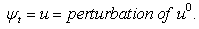
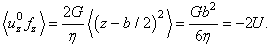
- Some fluids, as polymeric liquids, biological liquids, magma, are described by non-linear relations between the Cauchy stress tensor and strain-rate tensor and are called non-Newtonian fluids. The viscous and elastic properties of the non-Newtonian fluids are studied in a large number of papers - see [1-5].The Oldroyd-B model was introduced by J. Oldroyd [6] in 1950. Such models of rate type, as Maxwell upper convected and Oldroyd-B, can be used to describe the polymeric flows, often related with the secondary oil recovery process in a porous medium, approximated by the Hele-Shaw model. In this field we refer to [7-9].Numerical simulations of an Oldroyd-B flow in pipes are given in [10], [11]. Some results related with the stability of a thin film flow with visco-elasticity effect are given in [12].In this paper we consider the steady displacement of an Oldroyd-B fluid by air in a horizontal Hele-Shaw cell and study the interface stability. The Hele-Shaw plates are parallel with the xOy plane; the gap between is denoted by b. The Oz axis is orthogonal on the plates. We use the constitutive equations (2). The perturbations equations (14), (15), (24), (25) are derived from the basic equations (8), (11), (12). A scaling procedure allows us to neglect the vertical component w of the perturbed velocity - see relations (18) and (19). We use the Fourier mode decomposition (22) with amplitude f (z) for the perturbed velocities (u, v). An approximate formula of the amplitude f is given in formula (46), by using the particular flow geometry (a very “thin” Hele-Shaw cell). This allows us to perform a depth-average procedure in the dynamic boundary conditions (33) - (34) (i.e. Laplace law) as a final step, and we obtain the dispersion relation (52), given by a ratio. This explicit formula for the growth rate (in time) of perturbations in terms of the problem data is the novelty of our paper.The denominator of the ratio (52) contains a term depending on (a1 − a2), where a1, a2 are the relaxation and the retardation (time) constants appearing in the constitutive relations (2) of the Oldroyd-B fluid. When a1 = a2, our formula (52) is quite similar with the Saffman-Taylor formula [13] for a Newtonian liquid displaced by air (see the last part of section 5).Our dispersion relation shows us that the displacement process of an Oldroyd-B fluid by air can be more unstable, compared with the displacement of a Newtonian liquid by air, so the elasticity properties have a destabilizing effect - see section 6, in agreement with some numerical previous results (see [7] below).Wilson [7] considered a different scaling procedure and numerically solved a quite similar set of perturbation equations from which he obtained numerical values of the growth rate σ, for Deborah numbers near 1.Mora and Manna [8], [9] studied the linear stability of the displacement of a Maxwell upper-convected fluid and generalized non-Newtonian fluids in a Hele-Shaw cell and obtained numerical values for the growth rate of perturbations, in the range of large Deborah numbers.The growth rate (52) can be unbounded in the range of small Deborah numbers. The possible singularities may be related with the fractures observed in the flows of some complex fluids in Hele-Shaw cells - see [14-18].The paper is laid out as follows. The constitutive equations for the Oldroyd-B fluid are given in section 2. In section 3 we describe the basic flow and we obtain the equations of perturbations. In section 4 we describe the kinematic and dynamic boundary conditions on the interface air-liquid, that means the Laplace law, used also in [7]. The dispersion relation (52) is given in section 5. We conclude in section 6, where some plots are given, proving the destabilizing effect of the elasticity properties of the Oldroyd-B fluid.
2. The Oldroyd-B Fluid
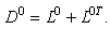
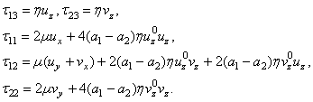
- We consider the following definitions. The extra-stress tensor, the fluid viscosity, the relaxation and retardation (time) constants and the pressure are denoted by τ, η, a1, a2, p.The 3 × 3 matrix containing the partial derivatives of the velocity components u, v, w is denoted by L and the strain-rate tensor is denoted by D:
 The flow equations are:
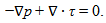 | (1) |
 | (2) |
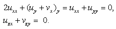
 where τt, Dt are partial time derivatives. As we consider a steady displacement, these time derivatives will be neglected.We consider an incompressible fluid, then we have the free divergence condition:
 | (3) |
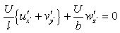
3. Basic Steady Flow and Perturbations
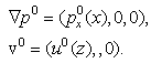
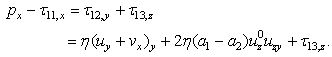
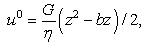
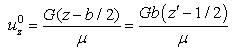
- We first consider the flow driven by the constant pressure gradients in the x, y directions and two velocities u, v depending only on z. The elements of this basic flow are denoted by the superscript 0. The subscripts denote the partial derivatives with respect to x, y, z. The basic pressure and velocity are denoted by
 | (4) |
 | (5) |
 | (6) |
 | (7) |
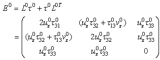
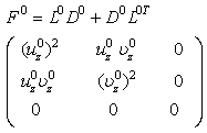
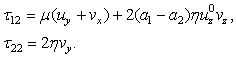
 of the basic extra-stress tensor are given in terms of the basic velocity components by the equations
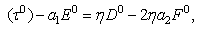 | (8) |
 | (9) |
 | (10) |
 = 0. Other components of the basic extra-stress tensor are
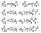 | (11) |
 are depending only on z, we have
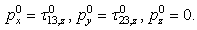 | (12) |
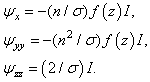
 | (13) |
 | (14) |
 = 0 - see the justification (21) below. The perturbed flow equations are
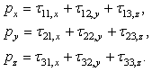 | (15) |
 | (16) |
 | (17) |
 | (18) |
 and because
 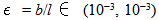 we can conclude
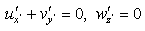 | (19) |
 | (20) |
 | (21) |
 | (22) |
 | (23) |
 Then from the formulas (14), (15), (17)1, (22) it follows
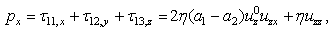 | (24) |
 | (25) |
 | (26) |
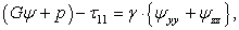
4. The Laplace Law
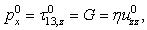
- We consider non-slip conditions for the velocities on the Hele-Shaw plates, then from the relations (13) we get
 | (27) |
 and
and  in the range
  We follow Wilson [7], then the pressure can depend on the time t:
 | (28) |
 | (29) |
 | (30) |
 The perturbed interface is
 | (31) |
 | (32) |
 | (33) |
 is the surface tension on the interface air-liquid and
  is the perturbation of the straight initial interface (31). The relation (32) is giving
 | (34) |
 in the plane xOy is approximated by
  The relations (31) - (34) are used also in Wilson [7].
5. The Dispersion Relation
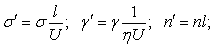
- We use the notation
 | (35) |
 | (36) |
 | (37) |
 | (38) |
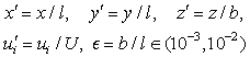
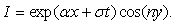
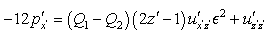
 appearing in the Fourier modes decomposition (11). For this we use our particular flow geometry and obtain the approximate formula (46) below.We introduce the dimensionless quantities
 | (39) |
 | (40) |
 then
then | (41) |
 then the last two relations and (24) are giving
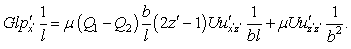 | (42) |
 and
and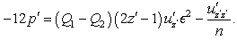 | (43) |
 the above relation (43) is giving
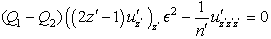 | (44) |
 and
and  is given in the relation (48) below.We can see that:- if
 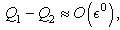 then
then  is verifying equation (44) with the precision order
  - if
- if then
then  is verifying equation (44) with the precision order
  We consider the following condition:
 | (45) |
 approximate solution
 | (46) |
 From (38) and the last two above relations it follows the dispersion relation
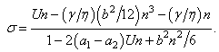 | (47) |
 | (48) |
 | (49) |
 in the denominator of the ratio (47). From (30) we have
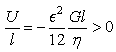 | (50) |
 and the condition (45) is giving
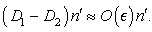 | (51) |
 | (52) |
 (that means
  ) we obtain an expression quite similar with the Saffman-Taylor formula for air displacing a Newtonian fluid with viscosity
  , but we have three new terms as follows:- the new term
  in the numerator, due to the meniscus curvature across the plates;- the new term
  in the denominator, due to the non-Newtonian effect;- the new term
  in the denominator, due to the fact that Fourier mode decomposition (22) does not allow us to neglect the derivatives with respect to
  .
.6. Conclusions
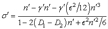
- We obtained an exact dispersion formula for the linear stability of an Oldroyd-B fluid displaced by air in a Hele-Shaw cell. The perturbations of the basic flow are verifying the very simple equations (14), (15), (17), (24), (25), (26).When a1 = a2, the obtained dispersion relation (52) is quite similar with the well-known Saffman-Taylor formula for a Newtonian fluid displaced by air in a Hele-Shaw cell:
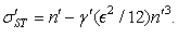 | (53) |
 Then our formula (52) becomes
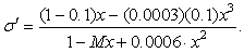 | (54) |
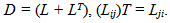
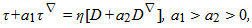
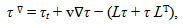
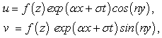
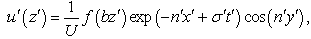
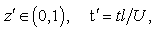
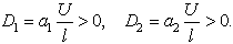
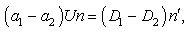
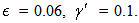
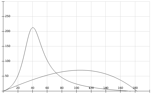
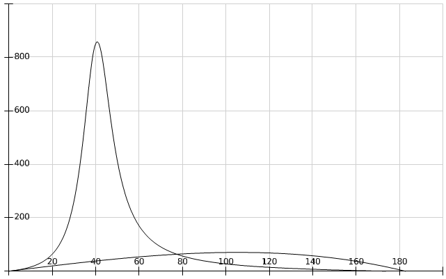
 and 2(D1 − D2).In Figure 2 we used the following values of order
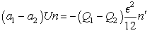
  (in agreement with the estimate (51)):M = 0.01, 0.02, 0.03, 0.04, 0.041, 0.042.We can see the non-Newtonian destabilizing effects.In Figures 3, 4 we used the valuesM = 0.045, 0.048.For M = 0.05 we get a blow-up of the growth rate (52), that means we have two real roots of the denominator in the ratio (54), because∆ = (0.05)2 − 4(0.0006) = 0.0001 > 0.These roots are giving a blow-up of the growth rate, which can be related with the fractures observed in the flows of some complex fluids in Hele-Shaw cells [14, 15, 17, 18], as we mentioned in Introduction. This phenomenon exceeds the linear stability frame and should be better analyzed by using a nonlinear theory.
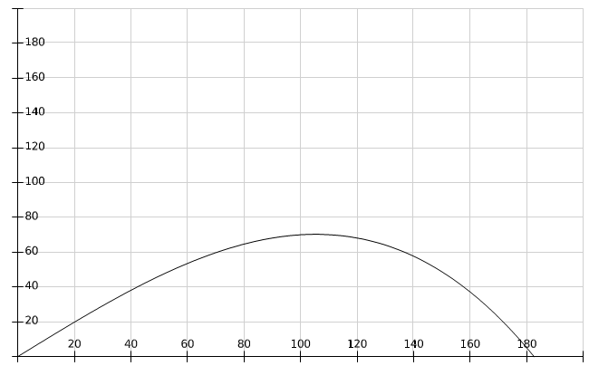 | Figure 1. Saffman-Taylor formula (53): 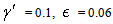 |
 | Figure 2. Eq. (54):  M = 0.01, 0.02, 0.03, 0.04, 0.041, 0.042 M = 0.01, 0.02, 0.03, 0.04, 0.041, 0.042 |
 | Figure 3. Formula (54):  M = 0.045 M = 0.045 |
 | Figure 4. Formula (54):  M = 0.048 M = 0.048 |
 - second, we considered the hypothesis (45) and neglected the terms of order
  in the relation (44).Then from this point of view, our dispersion formula (52) can be considered as an
  approximation of the growth rate.We emphasize that in the formula (52) we not neglected the terms of order
  and
and  which are multiplied with the dimensionless wave number
  or
or  We can see that, only for very small values
  of the wave numbers, our formula (52) is quite close to the Saffman-Taylor formula (53).