1. Introduction

The anaerobic respiration process is one of the attractive alternate for the economical reduction of the organic matter concentration in vegetables solids wastes [1-3]. Anaerobic digestion consists of a multitude of biochemical reaction in the series and in the parallel that occurs simultaneously [2, 4-6]. Mosey [7] and Kalyuzhni and Davlyatshina [8] developed the mathematical models which describes the kinetics of acidogenesis, ethanol degrading acetogenesis, acetogenesis, butyrate degrading acetogenesis, acetoclastic methanogenesis, hydrogenothrophic methanogenesis, bacterial decay, pH and various inhibitions of the mention steps. Mosche and Jordening [9] discussed the acetate and propionate degradation and inhibition. Masse et al. [10] studied the pre treatment of slaughterhouse wastewater at 25℃ for 5.5 h with 250mg/l of pancreatic lipase. Hu et al. [11] investigated the anaerobic digestion kinetics of ice cream water waste using monod and contois models. Aguilar et al. [12] studied the kinetic parameters of the total volatile acid degradation of source. Fang and Yu [13, 14] discussed the influence of influent concentration and temperature on the hydrolis of gelatinaceous wastewater.

Knobel and Lewis [15] developed a mathematical model in which in which the activity coefficients were calculated using the Debye-Hiicle theory and describing the anaerobic digestion of water waste with high concentration of sulphate. Gracia et al. [16] used first and second order kinetic models to describe the anaerobic digestion of livestock manure. The result obtain showed that the second model has both statically and physical meanings in the parameter values obtained. Munch et al. [17] developed the mathematical model for volatile acid production. Valentini et al. [18] compared the Michaelis -Menten substrate first order, substrate and biomass first order and substrate first order and biomass half order equations in the anaerobic degradation of cellulose particles of known size. Zainol et al. [19] carried out the kinetic evaluation of the different steps of anaerobic digestion (hydrolysis, acidogenic and methanogenic) process of banana stem waste using two stage system. The system consist of an anaerobic sequencing batch reactor for the first stage and an anaerobic fixed bed reactor for the second stage which is operating at Hydraulic retention times of nine days. In this paper we derive an approximate analytical expression for concentrations of the non-soluble organic matter, soluble organic matter, TVA consumption and, methane formation in terms of the kinetic parameters k₁-k₇ using new Homotopy perturbation method.

2. Mathematical Formulation of the Problem

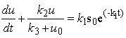
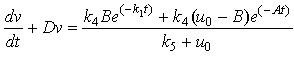
Taking into account the characteristics of banana stem waste (BSW) and the experimental results were obtained, the following hypothesis was assumed [19]: (i). The insoluble organic matter or volatile suspended solids were first transformed to soluble organic matter following first-order kinetics. (ii). the dissolved organic matter resulting from the decomposition of the insoluble organic matter and initially present in the raw banana stem waste was transferred to volatile acids following a Michaelis-Menten kinetics model. (iii). the volatile acids resulting from the decomposition and initially present in the raw banana stem waste was transferred to methane and carbon dioxide following a Michaelis-Menten kinetics model. (iv). the disaster was assumed to be a completely mixed reactor. (v). with these assumptions, the rate equations of organic matter of the kinetic model including methane production can be expressed in the following differential equations [19]:

(1)

(2)

(3)

(4)

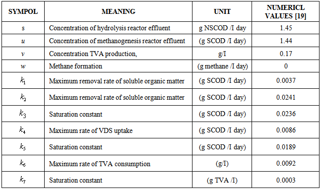
Where s is the non-soluble organic matter (g NSCOD/I day), u is soluble organic matter (g SCOD/I day), v is the TVA production (g/I day), w is the methane formation (g methane/I day). is the kinetic constant of the reaction, is the maximum removal rate of soluble organic matter, is the saturation constant, is the maximum rate of VDS uptake , is the saturation constant, is the maximum rate of TVA consumption, and is the saturation constant. These equations are solved for the following initial conditions.

(5)

3. Approximate Analytical Expression of the Concentration of Non-Soluble Organic Matter, Soluble Organic Matter, Tva Consumption and, Methane Formation Using New Homotopy Perturbation Method (Hpm)

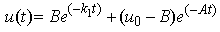
Non-linear phenomenon plays an important role in applied mathematical and physical science. Explicit solutions of the non-linear equations are the fundamental importance. Various methods for obtaining explicit solutions of non-linear equations have been proposed. Recently many authors have used the HPM for solving various problems and demonstrated the efficiency of the HPM for solving the non-linear problems in various physics and engineering problems [19-21]. This method is the combination of topology and classical perturbation techniques. He used the HPM to solve the Lighthill equation [22], the Diffusing equation [23] and the Blasius equation [24]. The idea has been used to solve non-linear boundary value problems, integral equations and many other problems. The Homotopy perturbation method [25-27] is very effective and simple. The HPM is unique in its applicability, accuracy, efficiency uses the imbedding parameter p as a small parameter and only a few iterations are needed to search for asymptotic solutions. Using this method, we can obtained the following approximate solution for the equations (1)-(4) (ref Appendix-A).

(6)

(7)

(8)

(9)

where the constant

(10)

Equations (6)-(9) satisfy the initial conditions (5). Equations (6)-(8) represent the new approximate analytical expression of concentration of hydrolysis reactor effluent , methanogenesis reactor effluent , acetic acid effluent from methanogenesis reactor and methane formation in terms of kinetic parameters.

4. Numerical Simulation

The non-linear differential equations (1)-(4), are also solved using numerical methods. The function pdex4 in Scilab software which is the function of solving the initial value problems for ordinary differential is used to solve this equation. Its numerical solution is compared with our approximate analytical result in Figure-1 and it gives a satisfactory agreement for all experimental values of the parameters ( and time days. The Scilab program is also given in Appendix-B.

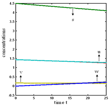Figure 1. Plot of concentrations of hydrolysis reactor effluent , methanogenesis reactor effluent , acetic acid effluent from methanogenesis reactor , methane formation verses time (day) using the Eqs. (5)-(8)

5. Discussion

Equations (6)-(9) are simple and closed-form of approximate analytical expression of the concentrations of hydrolysis reactor effluent , methanogenesis reactor effluent , acetic acid effluent from methanogenesis reactor , methane formation for various kinetic parameters . In Figs.1-11, the concentrations of hydrolysis reactor effluent , methanogenesis reactor effluent , acetic acid effluent from methanogenesis reactor , methane formation verses time t have been plotted for some fixed values of kinetic parameters. In Fig-1, our approximate analytical results () are compared with the numerical results [19]. Our approximate analytical result fit very well with the experimental result. Fig. 2 shows the concentration hydrolysis reactor effluents versus time t using Eq.6 for various values of kinetic constant . From this figure, we can see that the value of concentration decreases when time t increases with increasing values of _.

Figs. 3- 5 represent concentration methanogenesis reactor effluent u at the time t using Eq.7. From the Fig 3, it is observed that the concentration u increases when increases. In Fig. 4 and 5 the concentrations are plotted for various values of parameters and respectively. From these figuresit is inferred that value of concentration decreases when and increases.

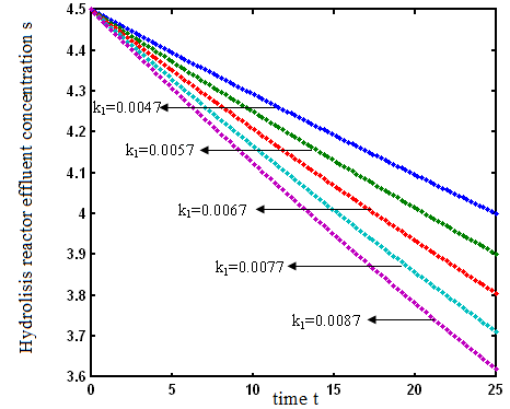Figure 2. Plot of concentration of hydrolysis reactor effluent s verses time t (day) for various values of parameters k1using the Eq. 5. (a) k1 = 0.0047; (b) k1 = 0.0057; (c) k1 = 0.0067; (d) k1 = 0.0077; (a) k1 = 0.0087

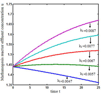Figure 3. Plot of concentration of Mathanogesis reactor effluent u verses time t (day) for various values of parameters k1 using the Eq.6. (a) k1 = 0.0047; (b) k1 = 0.0057; (c) k1 = 0.0067; (d) k1 = 0.0077; (a) k1 = 0.0087

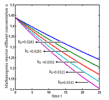Figure 4. Plot of concentration of Mathanogesis reactor effluent u verses time t (day) for various values of parameters k2 using the Eq. 6. (a) k2 = 0.0261; (b) k2=0.0281; (c) k2=0.0301; (d) k2=0.0321; (e) k2=0.0341

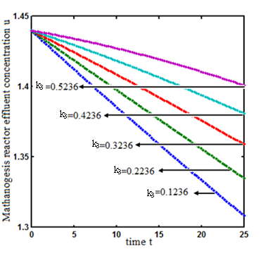Figure 5. Plot of concentration of Mathanogesis reactor effluent u verses time t (day) for various values of parameters k3 using the Eq. 6. (a) k3=0.1236; (b) k3 = 0.2236; (c) k3 = 0.3236; (d) k3 = 0. 0.4236; (e) k3 = 0.5236

In Figs. 6-9 we present the concentration of methanogenesis reactor v at time t using Eq.8. From Figs. 6 and 9 it is deducted that values of concentration increases when parameters and increases. From Fig.7 and 8 it is inferred that value of concentration decreases when parameters and increases.

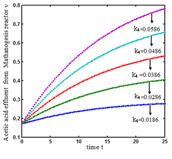Figure 6. Plot of concentration of Acetic acid effluent from Mathanogesis reactor v verses time t (day) for various values of parameters k4 using the Eq. 7. (a) k4 = 0.0186; (b) k4 = 0.0286; (c) k4 = 0. 0386; (d) k4 = 0.0486; (e) k4 = 0.0586

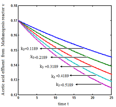Figure 7. Plot of concentration of Acetic acid effluent from Mathanogesis reactor v verses time t (day) for various values of parameters k5 using the Eq. 7. (a) k5=0.1189; (b) k5 =0.2186; (c) k5 =0.3189; (d) k5 =0.4189; (e) k5 = 0.5189

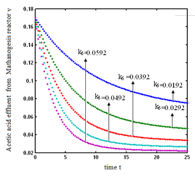Figure 8. Plot of concentration of Acetic acid effluent from Mathanogesis reactor v verses time t (day) for various values of parameters k6 using the Eq. 7. (a) k6 = 0.0192; (b) k6 = 0.0292; (c) k6 = 0.0392; (d) k6 = 0.0492; (e) k6 = 0.0592

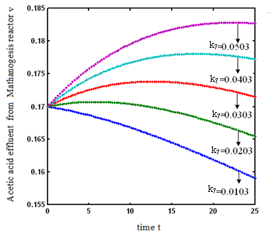Figure 9. Plot of concentration of Acetic acid effluent from Mathanogesis reactor v verses time t (day) for various values of parameters k7using the Eq. 7. (a) k7 = 0.0103; (b) k7 = 0.0203; (c) k7 = 0.0303; (d) k7 = 0.0403; (e) k7 = 0.0503

Figs. 10 and 11 represents concentration w for various values of and respectively. From these figures, it is observed that concentration methane formation w increases when saturation constant and increases.

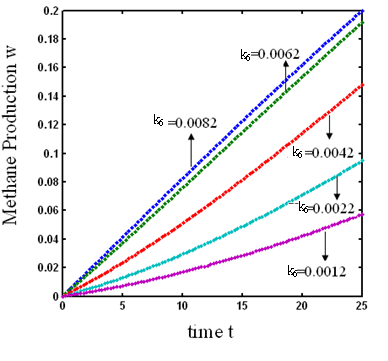Figure 10. Plot of concentration of Methane production w verses time t (day) for various values of parameters k6 using the Eq. 8. (a) k6 = 0.0082; (b) k6 = 0.0062; (c) k6 = 0.0042; (d) k6 = 0.0022; (e) k6 = 0.0012

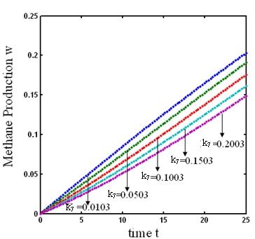Figure 11. Plot of concentration of Methane production w verses time t (day) for various values of parameters k7 using the Eq. 5. (a) k7 = 0.0103; (b) k7 = 0.0503; (c) k7 = 0.1003; (d) k7 = 0.1503; (e) k7 = 0.2003

6. Conclusions

A nonlinear time independent equation has been solved analytically using new Homotopy perturbation method. In this paper we have presented approximate analytical expression of the concentration of hydrolysis reactor effluent, methanogenesis reactor effluent, acetic acid effluent from methanogenesis reactor, methane formation for time days. The influence of the saturation constant on concentrations is also discussed.

ACKNOWLEDGEMENTS

This work is supported by the Department of Science and Technology (DST), Government of India. The authors are thankful to Shri. S. Natanagopal, Secretary, The Madura College Board and Dr. R. Murali, Principal, The Madura College (Autonomous), Madurai, Tamilnadu, India for their constant encouragement.

Nomenclature

Appendix

Appendix A: Approximate Analytical Solutions of the Equation (1)-(4) Using New Homotopy perturbation Method

In this appendix, we indicate how equations (6)-(9) in this paper are derived. Furthermore a new Homotopy was constructed to determine the solutions of (1)-(4) and the initial conditions are as follows:

Solving Eq.1, we get

(A1)

Substitute the values of Eq. A2 in Eq. 2 we get

(A2)

The Homotopy ofEqu.2 can be constructed as follows:

(A3)

The zeroth iteration of the above equation can be written as

(A4)

Solving the above equation using the initial condition, we get

(A5)

where the constant

(A6)

(A7)

Where the constant

(A8)

Solving the above equation using the initial condition we get

(A9)

Substitute the values of Eq.A9 in Eq.3 and using new HPM approach, we get the zeroth iteration equation as

(A10)

Solving the above equation using the initial condition, we get

(A11)

Appendix B: Matlab Program to Find the Numerical Solution of Eqs.(1)-(4)

function main1

options= odeset('RelTol',1e-6,'Stats','on');

Xo = [4.5;1.44;0.17;0];

tspan = [0,50];

tic

[t,X] = ode45(@TestFunction,tspan,Xo,options);

toc

figure

hold on

%plot(t, X(:,1))

%plot(t, X(:,2))

%plot(t, X(:,3))

plot(t, X(:,4))

return

function [dx_dt]= TestFunction(t,x)

k1=.0037;k2=0.0241;k3=0.0236;k4=0.0086;k5=0.0189; k6=0.0092;k7=0.0003;

dx_dt(1)=-k1*x(1);

dx_dt(2)=k1*x(1)-((k2*x(2))/(k3+x(2)));

dx_dt(3)=((k4*x(2))/(k5+x(2)))-((k6*x(3))/(k7+x(3)));

dx_dt(4)=((k6*x(3))/(k7+x(3)));

dx_dt = dx_dt';

return