Bright O. Osu1, Joy I. Adindu-Dick2
1Department of Mathematics, Abia State University, Uturu, Nigeria
2Department of Mathematics, Imo State University, Nigeria
Correspondence to: Bright O. Osu, Department of Mathematics, Abia State University, Uturu, Nigeria.
| Email: |  |
Copyright © 2015 Scientific & Academic Publishing. All Rights Reserved.
Abstract
We studied the rate of returns on investment as the net gain in wealth over the cumulative investment in continuous time. Dynamic asset allocations are continuously rebalanced so as to always keep a fixed constant proportion of wealth invested in various assets at each point in time play a fundamental role in the theory of optimal portfolio strategy. We proved that: (i) the limiting distribution of this measure of return is gamma distribution if the returns follow a geometric Brownian motion; (ii) if returns follow Weibull distribution, then it results to asymptotic power-law behavior of assets returns. For example, the mean return on investment is maximized by the same strategy that maximizes logarithm utility which is also known to minimize the exponential rate at which wealth grows and the return from this policy turns out to have stochastic dominance properties as well. We consider the logistic function in large market financial crashes corresponding to values of packing dimension of  by the fractal dispersion of Hausdorff measure prior to market signal with constraint of a zero heat capacity, the existence of a unique solution to the associated Hausdorff is established and optimal policy is characterized. Also advocated is a procedure for locating optimal market crises signal relative to the heat equation to give an early warning.
Keywords:
Optimal policy, Contingent claim, Power Law, Hausdorff measure, Market signal, Fractal dispersion
Cite this paper: Bright O. Osu, Joy I. Adindu-Dick, Optimal Policy on the Possible Rate of Returns of Contingent Claim by Fractal Dispersion on Hausdorff Measure to Market Signal, Applied Mathematics, Vol. 5 No. 1, 2015, pp. 1-6. doi: 10.5923/j.am.20150501.01.
1. Introduction
Ethier et al, [2] studied the rate of return on investment in discrete time gambling method, where the total return on the individual gambler is assumed to follow a random walk. They also showed that the asymptotic distribution of the return, as the mean increment in the random walk goes to zero is a gamma distribution. Also Kelly (1956) in Thorp, [11] observed the relationship between the logarithm of wealth and expected asymptotic rate at which wealth compounds. The object is to let one know how one should invest in each equities of ones highly diversified stocks portfolio to maximize the capital growth. In finance, the rate of return (ROR) which is known as return on investment (ROI) is the ratio of money gained or lost whether realized or unrealized on an investment, relative to the amount of money invested. The amount of money gained or lost may be referred to as interest, profit/loss, gain/loss or net income/loss. There are several ways to determine ROI, but the most frequently used method is net gain divided by total assets. Constant proportions investment strategies also play a fundamental role in portfolio theory. Under these policies, an investor follows a dynamic trading strategy that continually rebalances the portfolio so as to always allocate fixed constant proportions of the investor’s wealth across the investment opportunities. These strategies are widely used in practice and are also referred to as continuously rebalanced strategy [9]. Given the fundamental nature of policies in theoretical portfolio practice, it is of interest to know what the stochastic behavior of the rate of return on investment (RROI), defined as the net of gain over the cumulative investment [3]. Merton, [5] introduced the setting in the continuous time financial model as used in Black-Scholes, [1].In this paper, we obtain some limit theorems for RROI which allows us to compare and derive some specific optimality properties for certain portfolio strategies. We also established and proved that the return on investment for such policies converges to a limiting stochastic distribution and the result provides a basis upon which to compare different strategies on Hausdorff measure prior to the heat equation to locate market crises and give early warning.
2. The Rate of Return from Total Investment
The rate of return on investment is defined as the ratio of net gain in wealth over the cumulative investment. Our interest here is the rate of return from the total investment (RROI), which for the fixed policy will be denoted by the process  Hence
Hence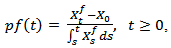 | (2.1) |
which is equivalent to the least square estimator  studied by Hu, et al [4] on the continuous parametric estimation of observed fractional Ornstein-Uhlenbeck process
 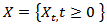 defined as
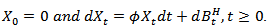 | (2.2) |
 is a fractional Brownian motion with Hurst parameter
  given as
 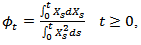 | (2.3) |
Where  is a measure of the wealth it takes to finance a gain. If
  is large; it means that the investor is accumulating gains at a faster rate than if it is small. Note that if we divide the numerator and the denominator by t in equation (2.1) we also interpret
  as the average net gain over the average wealth level.Theorem 2.1If the returns of contingent claim
 follow geometric Brownian motion
 , then the resulting distribution is Gamma distribution, that is,
 ProofRecall that
 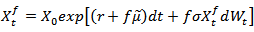 then
then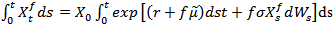 | (2.4) |
From geometric Brownian motion, | (2.5) |
and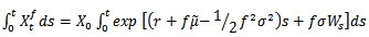 | (2.6) |
Substitute (2.5) and (2.6) in (2.1) to get which implies
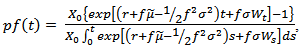 and simplifies to
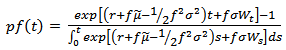 | (2.7) |
If  we have that from equation (2.7) it shows that for that policy under which the total wealth is always invested in the risk-free asset is
 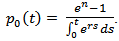 But
But  so that
 If
If  then
then  is the risk free interest rate as expected but if
  the rate of return on investment (RROI) process
  is complicated and does not yield to a simple direct analysis.NOTE: a random variable
  gamma
gamma  means that X is a random variable with density function
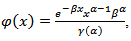 with
with  and the
  And for any fixed proportion that satisfies
 all
all  , the (RROI) process
 converges
  in distribution to random variable which has a gamma distribution, where
  is the constant vector given by
 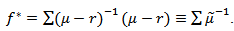 If
If  is a constant vector for all
  such a policy is called constant proportion policy which is the optimal investment policy for any interesting objective function. A constant vector is also optimal policy for other objective criteria, such as minimizing the expected time t to reach a given level of wealth as well.Specifically, as
  we have
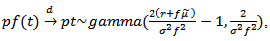 | (2.8) |
where  denotes convergence in distribution.Therefore to get the expectation of
  we have
 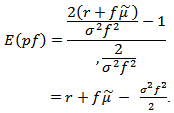 | (2.9) |
The expectation in (2.9) should not be confused with the ratio of the expected gain to the expected total investment which for any  is equal to
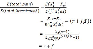 | (2.10) |
Theorem 2.2If the returns  as defined in (2.1) follow Weibull randomvariates
 , then the resulting distribution
  follows asymptotic power-law.ProofLet
 be distributed according to the following probability density function
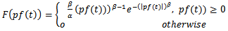 | (2.11) |
where  are the mean and the shape parameters of the Weibull distribution (2.11).If
  has the Weibull density function, then
  has the exponential density function with
  as (using the formula in [7]);
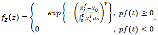 | (2.12) |
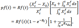
Thus the optimal investment strategy is (see [8]);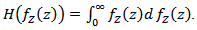 | (2.13) |
That is 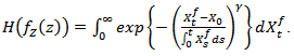 | (2.14) |
But  (where
  is as in (2.4) or (2.6)), so that
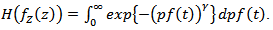 Hence the optimal strategy is the asymptotic power-law;
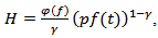 | (2.15) |
where is the fractal exponent given by (see [6])
  with
with  a Bessel function given as
  and
and  the singularity strength
3. Optimal Growth Policy and Stochastic Dominance
Here we can see that the quantity (2.8) is maximized by the strategy that invests as much as possible in the risky asset. The mean of (2.7), is maximized at a finite value  | (3.1) |
which is the same policy that is optimal for maximizing logarithmic utility of wealth at a fixed terminal time and hence for maximizing exponential rate of growth. Notice that the mean of the limiting distribution of (RROI) process is maximized at the value  with resulting mean
  for this strategy the RROI,
  satisfies
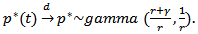 | (3.2) |
In fact, the distribution characterization of the limiting RROI allows for some-what stronger statement, in terms of stochastic orderings. Suppose that for two random variables, X,Y we say that 
 This is equivalent to say that
  for all increasing convex function
  and is referred to as the increasing convex ordering. We also say that (provided the expectations are finite) this is equivalent to saying that
  for all increasing concave function
  and is hence referred to as the increasing concave ordering.We let
  denote the RRIO obtained from using the policy
  defined in (2.9) and let
  be the RROI. From any other constant proportion strategy
  where c is an arbitrary constant, the following hold
 Equation (a) is in effect for investor with greater relative risk aversion while equation (b) is in effect for an investor with less relative risk aversion. Then for a proportional strategy
  where
where  is the optimal policy of (2.7), the relationship
  holds if and only if C satisfies
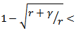
 Showing that the only type of constant proportion policy (other than
  for which RROI is stochastically dominated by the optimal growth policy is one that is shorting the stock to the degree required by
  To establish equation (2.1) in section 1 above, we have that the process
  does not admit a simple direct analysis, there is a related markov process amenable to analysis which holds the key for the limiting behavior of
  specifically the
  0 defined by
 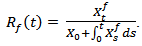 | (3.3) |
If t = 0 we have  also we will first show that the limiting behavior of
  is equivalent to the limiting behavior of
  But our interest here is to show the limiting behavior of the RROI process
  We show that the diffusion process
  whose limiting behavior can be analyzed.Suppose that for random variable
  we have
 Then for any
 we have

 | (3.4) |
where  is the linear Brownian motion defined by
 Note that
  hasa positive drifts which implies that
 as well as
  Equation (2.1) will be completely establish if we can prove that
  for some random variable
  with
with  Lemma 3.1: For some fixed proportion investment policy
  the process
  follows the stochastic differential equation
 | (3.5) |
 is a temporary homogeneous diffusion process with drift function
  and diffusion function
 ProofLet
  be the cumulative wealth investment process, also let
  Since
Since  is a process of bounded variation, its Ito’s rule show that
  so applying Ito’s rule to
  gives
gives 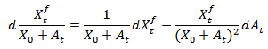 which upon substitution gives
 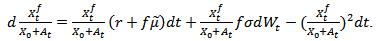 | (3.6) |
The result is equivalent to (3.5). Here, the policy is maximized by a strategy that invests as much as possible in the risky asset and the total return from this policy turns out to have stochastic dominance property as well. This continuous stochastic process can be used for modeling random behavior that evolves over time like fluctuation in an asset price.
4. Application on Logistic Financial Fractal Dispersion Function of the Hausdorff Priorto Crash Market Signal
One of the several distinct techniques of investigating the size of subsets of zero market in  is the notion of packing dimension due to Taylor and Triort, [10].Packing dimension is defined via the packing measure as a class φ of monotone functions h
  which is non decreasing, right continuous satisfying h(0+) = 0 and for which there is a constant.
 | (4.1) |
We obtain the packing dimension by two definitions. First, we defined a pre-measure 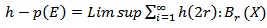 | (4.2) |
disjoint  Where
Where  denotes the open ball centered on X radius r Eq(4.2) is not an outer measure because it is not count ably Sub-additive. However it leads to an outer measure by defining
 | (4.3) |
which can be thought of as a generalization of Hausdorff measure using maximal packing of E by balls, so that if h(s)  then h –p( ) on
  is n-dimensional Hausdorff measure. Thus to measure the Borel subset of
  we need
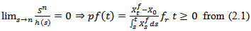 | (4.4) |
So that if  there is a unique value of
  for which the packing measure h- P(E) drops from infinity to zero.This in turn means that E is less occupied than if it were
  dimensional. For
  We define the next Dim E as
  | (4.5) |
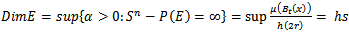 | (4.6) |
which denotes the packing dimension E.The underlying assets is paying nontrivial continuous dividends with an annualized yield  A holder of the underlying asset receives a dividends yield
  over any time interval with length
  Paying dividends leads to the asset price decrease
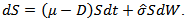 | (4.7) |
Comparing equations (3.5) and (4.7) implies that  After an elapse of time
  the value of the portfolio will change by the rate
  in view of the dividend received on h units held. Using Ito’s lemma for
  we conclude with the equation
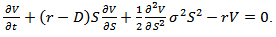 | (4.8) |
Using a new function (where
  are some constants) and the transformation
  we have;
 which is substituted in (4.8) to get ;
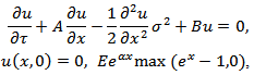 | (4.9) |
where  and
and 
 By setting

 that (4.9) reduces to finding the solution of the Cauchy problem
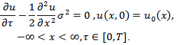 | (4.10) |
Consider a market comprising of  unit of wealth in long position (expected) and
  unit of the wealth in short position (actual), at time
  the market value is assumed to be
  after an elapse the value changes by the amount and the Hausdorff measure in this case is to determine which subsets of
  is the n-dimensional Euclidean space) are of zero heat capacity (that is where there is no market signal and hence market crash) with respect to the heat equation
  | (4.11) |
A solution  to the Cauchy problem (4.10) is given by the Green’s formula
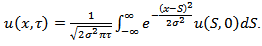 | (4.12) |
Equation (4.12) gives us the idea that the transition density of the Brownian motion in  is just the heat kernel (for
 which satisfies the heat equation (4.11). The measure zero is equivalent to the heat capacity zero on the hyper plane. It therefore follows that the solution of (4.8) is given as;
 | (4.13) |
The market crash (bubble) source gives rise to a  which assigns a value to a portfolio
  to each point of
  through a generating kernel
  so that on a positive market strategy
  on
on  is the portfolio growth rate if it is finite on a dense subset of
5. Conclusions
Equations (2.8) and (2.15) reveal that: (i) if assets returns follow a geometric Brownian motion, then the limiting distribution is gamma distribution, conversely (ii) if returns follow Weibull distribution, then it results to asymptotic power-law behavior. Furthermore the optimal strategy (2.15) depends on which in turn depends on
 (the singularity strength).
  as
as  and
and  (the optimal claims) increases without bound. As
  and
and  decrease constantly with
  Given (3.1), we have
  (the square of the correlation coefficient) and
  The policy is maximized by a strategy that invest as much as possible in the risky asset and the total return from this policy turns out to have stochastic dominance property as well. This continuous stochastic process can be used for modeling random behavior that evolves over time like fluctuation in an asset price and With Hausdorff measure and the heat equation via packing dimension
  and
and  there is no market signal as it tends to zero hence the market is likely to crash at that point indicating shortfall on the wealth investment. The exact packing dimension is determined for subset of
  for which
  is unbounded for
  Where
Where  is n-dimensional Euclidean space. (size of the market)And for analysis of subset of B of
  of Zero Hausdorff measure, it is appropriate to assume that
  So that if
  but
but  turns out to be either zero or infinity.
References
| [1] | Black, F. and Scholes, M. The Pricing of Option and Corporate Liabilities: Journal of Political Economy 81, (1973), 637-654. |
| [2] | Ethier, S N. and Tavare, S. The Proportional Bettor’s Return on Investments: Journal of Applied Probability 20(3), (1983), 563-573. |
| [3] | Hakansson, N.H., Optimal Investment and Consumption Strategies under Risk for a class of Utility Function: Econometrica 38(5), (1970), 587-607. |
| [4] | Hu Y. and Nualart D. Parameter Estimation for Fractional Ornstein-Uhlenbeck Process: Statistics and Probability Letters 80, (2010), 1030-1038. |
| [5] | Merton, R. C. Continuous-Time Finance: Basil Blackwell Inc., Cambridge, Ma, (1990). |
| [6] | Osu, B. O. and Adindu-Dick, J. I. Optimal Prediction of the Expected value of Assets under Fractal scaling exponent. To appear in MathSJ (2014). |
| [7] | Olkin, I., Gloser, I.J. and Derman, C. Probability models and Applications. Macmillian Publishing co, Inc. New York (1980). |
| [8] | Okoroafor, A. C. and Osu, B. O. An Empirical Optimal Selection Model. Afri. J. Math. Comp. Res. 2(1) (2009): 001-005. |
| [9] | Perold, A.F. and Sharpe, W.F., Dynamic Strategies for Asset Allocation: Reprinted from Financial Analyst Journal (1998), 16-27. |
| [10] | Taylor S.J. and Triort C., Packing Measure and its Evaluation for a Brownian path. Trans. Am. Math. Soc., 288: (1985), 679-699. |
| [11] | Thorp, E. O., Portfolio Choice and Kelly Criterion: Proceedings of the Business and Economics Section of the American Statistical Association, (1971), 215-224. |
 Abstract
 Reference
 Full-Text PDF
 Full-text HTML