1. Introduction

According to Britannica Online Encyclopedia (2011): “A bank is an institution that deals in money and its substitutes and provides other financial services”. Banks accept deposits, make loans and derive a profit from the difference in the interest rates charged. Banks are critical to our economy. The primary function of banks is to put their account holders’ money to use in other to optimize profit, by lending it out to others who can then use it to buy homes, do businesses, send kids to school, etc.

When you deposit money in the bank, your money goes into a big pool of money along with everyone else’s and your account is credited with the amount of your deposit. When you write checks or make withdrawals, that amount is deducted from your account balance. Interest you earn on your balance is also added to your account.

Number of studies have examined bank performance in an effort to isolate the factors that account for interbank differences in profitability. These studies fall generally into several categories. One group has focused broadly on the tie between bank earnings and various aspects of bank’s operating performance. A second set of studies has focused on the relationship between bank earnings performance and balance sheet structure. Another body has examined the impact of some regulatory, macroeconomic or structural factors on overall bank performance. The term bank structure is frequently used when referring to the characteristics of individual institutions. Individual bank characteristics such as the portfolio composition, and the scale and scope of operations, can affect the costs at which banks produce financial services. Market structure, measured by the relative size and number of firms, can influence the degree of local competition, and by extension, the quality, quantity, and price of financial services ultimately available to bank customers.

Bourke (1986) indicated that the determinants of commercial bank Profitability can be divided into two main categories namely the internal determinants which are management controllable and the external determinants which are beyond the control of the management of these institutions.

The internal determinants can be further subdivided as follows:

Ø Financial Statements variables

Ø Non-financial statement variable

The Financial statement variables relate to the decisions which directly affect the items in a balance sheet and profit & loss accounts. On the other hand, the nonfinancial statement variables involve those factors which do not have a direct impact on the financial statements. The external determinants on the other hand can be listed as follows

Ø Financial De-regulations

Ø Impact on competitive conditions

Ø Concentration

Ø Market Share

Ø Interest Rate on profitability

Ø Ownership

Ø Scarcity of Capital and Inflation

Banks create money in the economy by giving loans to their customers. These loans given to customers are usually associated with risk of non-payment. The amount of money that banks can lend is directly affected by the reserve requirement set by Federal Reserve or the Central Bank (ie. Bank of Ghana). Monetary and Exchange Rate Management in Ghana-Bank of Ghana (2011): “The reserve requirement is a ratio of cash to total deposits that a bank must keep. This is used for both prudential and monetary management purposes. During the period of direct controls, they were used as a supplement to credit controls. The reserve requirement ratio has evolved from its highest of 27% in 1990 to 10% in 1996 and its current level of 8% since 1997”. Since banks optimize profit through deposits and loans given to their customers. These loans are restricted by the bank’s reserve requirement and the bank also stands the risk of non-payment on the part of the customer. Therefore, there is a need for prudent management of these financial risks though the banks opt to make profit to be operational.

Therefore, the paper seeks to determine the Optimal Profit of Bank X Tamale in the areas of interest from loans such as Revolving Term Loans, Fixed Term Loans, Home Loans, Personal VAF, Vehicle and asset Finance as well as interest derived from Current Accounts, ATM withdrawals, Cheque Books and Counter Cheques of at least 90 customers for the period of six (6) months from November, 2011 to April, 2012. This problem of profit optimization of Stanbic Bank, Tamale is modeled as a Linear Programming Problem (LPP) and the resulting LPP is then solved using the Revised Simplex Method (RSM).

1.1. Linear Programming

Linear Programming is a subset of Mathematical Programming that is concerned with efficient allocation of limited resources to known activities with the objective of meeting a desired goal of maximization of profit or minimization of cost. In Statistics and Mathematics, Linear Programming (LP) is a technique for optimization of linear objective function, subject to linear equality and linear inequality constraint. Informally, linear programming determines the way to achieve the best outcome (such as maximum profit or lowest cost) in a given mathematical model and given some list of requirement as linear equation. Although there is a tendency to think that linear programming which is a subset of operations research has a recent development, but there is really nothing new about the idea of maximization of profit in any organization setting i.e. in a production company or manufacturing company. For centuries, highly skilled artisans have striven to formulate models that can assist manufacturing and production companies in maximizing their profit, that is why linear programming among other models in operations research has determine the way to achieve the best outcome (i.e. maximization of profit) in a given mathematical model and given some list of requirements. Linear programming can be applied to various fields of paper. Most extensively, it is used in business and economic situation, but can also be utilized in some engineering problems. Other industries such as transportation, energy, telecommunications and production or manufacturing companies use linear programming for maximization of profit or minimization of cost or materials. To this extent, linear programming has proved useful in modeling diverse types of problems in planning, routing and scheduling assignment.

Tucker (1993) noted linear programming is a mathematical method developed to solve problems related to tactical and strategic operations. Its origins show its application in the decision process of business analysis, funds. Although the practical application of a mathematical model is wide and complex, it will provide a set of results that enable the elimination of a part of the subjectivism that exists in the decision-making process as to the choice of action alternatives Bierman and Bonini (1973).

1.2. Background to the Paper

As banks device means to optimize profit, there are always associated financial risk. Ampong (2005) stated in Reserve Requirements in Bank - “Bank of Ghana stated that the Banking Act, 2004 which has passed through parliament indicates that:

A bank at times while in operation maintains a minimum capital adequacy ratio of 10%.

The capital adequacy ratio shall be measured as capital base of the bank to its adjusted assets base in accordance with regulations made by the bank of Ghana.”

The central bank is concerned about the possibility of a banking crisis resulting from the lack of adequate foresight in the actions of an individual bank. A bank capital reserve can fall dangerously too low hence fail to meet the operational requirements of its customers. When this unfortunate situation happened in the banking sector, the panicked customers will rush to the bank to cash their accounts. Some banks might need a higher capital adequacy requirement while others might need something much lower. In nominal terms 10% capital requirement for, say, Bank X Tamale could be the market capitalization of about five (5) Rural Banks combined.

In the above, it is quite obvious that while a bank opt to optimize profit through deposits, loans, interest rates charged etc., the bank should be mindful of how much is kept in the capital reserve and this must be determined by a specific risk conditions.

1.3. Statement of the Problem

Optimizing Profit in Bank X Tamale in the areas of interest from loans such as Revolving Term Loans, Fixed Term Loans, Home Loans, Personal VAF, Vehicle and asset Finance as well as interest derived from Current Accounts, ATM withdrawals, Cheque Books and Counter Cheques of at least 90 customers for the period of six (6) months from November, 2011 to April, 2012 became necessary as a result of keen competition among banks and each bank is much interested in determining its profit margin quarterly, half yearly or per year. Also, it is quite obvious that while a bank opt to optimize profit through deposits, loans, interest rates, etc, the bank should be mindful of how much is kept in the capital reserve. These problems have therefore provoked this paper on optimizing profit in the bank, a case paper of Bank X Tamale.

1.4. Organization of the Paper

The first section focuses on the introduction to the paper and deals with the background to the paper, the statement of the problem, and organization of the paper. The second section deals with the literature review. This provides a theoretical frame work within which the paper is located and some related research findings. Section three highlights on the methodology, this includes modeling the problem of profit optimization of Bank X Tamale as Linear Programming Problem; determination of the optimal profit using Revised Simplex Algorithm and providing sensitivity analysis of the problem of profit optimization. Section four provides for the results of the data analysis and discussion of the result whilst the final section provides the conclusion of the paper.

2. Related Literature Review

This chapter opens with a theoretical framework within which the paper is located and related research findings. The chapter centered on various reviews on Profit Maximization in the Bank, Linear Programming (LP) as an effective tool for Profit Optimization; how the Revised Simplex Method (RSM) is used to solve a Linear Programming problem (LPP) and related research findings on Sensitivity analysis.

2.1. Reviews on Profit Maximization in the Bank

Allen and Mester (1999) investigate the sources of recent changes in the performance of U.S. banks using concepts and techniques borrowed from the cross-section efficiency literature. Their most striking result is that during 1991-1997, cost productivity worsened while profit productivity improved substantially, particularly for banks engaging in mergers. The data are consistent with the hypothesis that banks tried to maximize profits by raising revenues from the products the bank render ( such as Loans, Current Accounts charges, ATM charges, etc) as well as reducing costs, and that banks provide additional services or higher service quality that raised costs but also raised revenues by more than the cost increases.

The U.S. Bureau of Labor Statistics (BLS) (1997) developed a labor productivity measure for maximizing profit in the commercial banking industry. They measure physical banking output using a “number-of-transactions” approach based on demand deposits (number of checks written and cleared, and number of electronic funds transfers), time deposits (weighted index of number of deposits and withdrawals on regular savings accounts, club accounts, CDs, money market accounts, and IRAs), ATM transactions, loans (indexes of new and existing real estate, consumer installment, and commercial loans, and number of bank credit card transactions), and trust accounts (number of these accounts), each weighted by the proportion of employee hours used in each activity. Employee labor hours are used as the denominator of the productivity index, although the BLS also computes an output per employee measure. For later comparison to their results and those of other research studies of labour productivity measure for profit maximization in the bank.

Rwanyaga (1996) carried out research work on Bank of Africa on things that affect profit levels in the bank. Regarding the paper findings, it was revealed that cash management in bank of Africa affects profitability levels. The findings also showed that the bank employs several cash management techniques in order to reduce fraud of cash in the bank. The paper also showed that profitability levels were high in the bank. The researcher recommended that there is a need for deploying a cash management system which involves support and coordination among multiple departments. Banks need to pick the right cash management provider who can coordinate the physical and technological installation of the system can significantly expedite and smooth the process of ensuring profit maximization. Each department should carefully consider features and functionality that will be required for a successful deployment and utilization of cash management which also increases profitability.

Lassila (1996) using a marginalistic approach that borrowing at high interest rates at the Central Bank in order to grant lower-interest loans can be consistent with straightforward short-term profit maximization for the bank. These phenomena simply result from the fact that the deposits received depend on the loans made, and, consequently, by borrowing at the Central Bank for credit expansion the bank generates sufficient additional deposits (which it invests in proper options) to make the borrowing profitable in spite of the high interest rate. Similarly, Cohen and Hammer (1996) Practitioners often argue that profit maximization is not an operational criterion in bank planning, and contend that maximization of a bank's deposits at the end of the planning horizon should be used instead. Their main argument is that short-term profit maximization is not consistent with the banks' long-term objectives. For example, in their opinion, short-term profit maximization gives no motivation for credit expansion. .

Laeven and Majnoni (2003) argue that risk can be incorporated into efficiency studies via the inclusion of loan loss provisions. That is, “following the general consensus among risk agent analysts and practitioners, economic capital should be tailored to cope with unexpected losses and loan loss reserves should instead buffer the expected component of the loss distribution. Consistent with this interpretation, loan loss provisions required to build up loan loss reserves should be considered and treated as a cost; a cost that will be faced with certainty over time but that is uncertain as to when it will materialize” (pp. 181). Among the earlier research that incorporated and studied the impact of nonperforming loans on bank efficiency are those of by Hughes and Mester (1993, 1998), Hughes et al. (1996, 1999) and Mester (1997), who included the volume of non-performing loans as a control for loan quality in studies of U.S. banks. Berg etal. (1993) on the other hand included loan losses as an indicator of the quality of loan evaluations in DEA paper of Norwegian bank productivity.

Shelagh Hefternan (1996) insisted that the banking world is changing rapidly; the strategic priority has shifted away from growth and size alone towards a greater emphasis on profitability, performance and value creation within the banking firm. The performance of the banks decides the economy of nation. If the banks perform successfully, the economy of nation must be sound, growing and sustainable one.

2.2. Linear Programming (LP)

Linear Programming was developed as a discipline in the 1940’s, motivated initially by the need to solve complex planning problems in war time operations. Its development accelerated rapidly in the post war periods as many industries found its valuable uses for linear programming. The founders of the subject are generally regarded as George B. Dantzig, who devised the simplex method in 1947, and John Von Neumann, who establish the theory of duality that same year. The noble price in economics was awarded in 1975 to mathematician Leonid Kantorovich (USSR) and the economist Tjalling Koopmas (USA) for their contribution to the theory of optimal allocation of resources, in which linear programming played a key role.

Many industries use linear programming as a standard tool, e.g. to allocate a finite set of resources in an optimal way. Example of important application areas include Airline crew scheduling, shipping or telecommunication networks, oil refining and blending, stock and bond portfolio selection. The problem of solving a system of linear inequality also dates back as far as Fourier Joseph (1768 – 1830) who was a Mathematician, Physicist and Historian, after which the method of Fourier – Motzkin elimination is named. Linear programming arose a mathematical model developed during the Second World War to plan expenditure and returns in other to reduce cost to the army and increase losses to the enemy. It was kept secret for years until 1947 when many industries found its use in their daily planning. The linear programming problem was first shown to be solvable in polynomial time by Leonid Khachiyan in 1979 but a large theoretical and practical breakthrough in the field came in 1984 when Narendra Karmarkar (1957–2006) introduced a new interior point method for solving linear programming problems.

Many applications were developed in linear programming these includes: Lagrange in 1762solves tractable optimization problems with simple equality constraint. In 1820, Gauss solved linear system of equations by what is now called Gaussian elimination method and in 1866, Whelhelm Jordan refined the method to finding least squared error as a measure of goodness-of-fit. Now it is referred to as Gausss-Jordan method. Linear programming has proven to be an extremely powerful tool, both in modelling real-world problems and as a widely applicable mathematical theory. However, many interesting optimization problems are nonlinear. The studies of such problems involve a diverse blend of linear Algebra, multivariate calculus, numerical analysis and computing techniques. The simplex method which is used to solve linear programming was developed by George B. Dantzig in 1947 as a product of his research work during World War II when he was working in the Pentagon with the Mil. Most linear programming problems are solved with this method. He extended his research work to solving problems of planning or scheduling dynamically overtime, particularly planning dynamically under uncertainty. Concentrating on the development and application of specific operations research techniques to determine the optimal choice among several courses of action, including the evaluation of specific numerical values (if required), we need to construct (or formulate) mathematical model Dantzig (1963), Hiller et al (1995), Adams(1969).

The development of linear programming has been ranked among the most important scientific advances of the mid-20th century, and its assessment is generally accepted.

2.2.1. Applications of LP for Profit Maximization in the Bank

Wheelock and Wilson (1996) used the linear programming approach to investigate bank productivity growth, decomposing the change in productivity into its change in efficiency and shift in the frontiers (profit). They found that larger banks (assets over $300 million) experienced productivity growth between 1984-1993, while smaller banks experienced a decline. Average inefficiency remained high in the industry, since banks were not able to adapt quickly to changes in technology, regulations, and competitive conditions. Similarly, Alam (1998) used linear programming techniques to investigate productivity change in banking using a balanced panel of 166 banks with greater than $500 million in assets and uninterrupted data from 1980 to 1989. As in Wheelock and Wilson, productivity change was decomposed into its two components: changes in efficiency and shifts in the frontier (profit). Bootstrapping methods were used to determine confidence intervals for the productivity measure and its components. The findings were that productivity surged between 1983 and 1984, regressed over the next year, and grew again between 1985 and 1989. The main source of the productivity growth was a shift in the frontier rather than a change in efficiency.

Veikko, Timo and Jaako (1996) an intertemporal linear programming model for exploring optimal credit expansion strategies of a commercial bank in the framework of dynamic balance sheet management assuming that it is both technically feasible and economically relevant to establish a linear relationship between the bank's credit expansion and the deposits received by the bank induced by the credit expansion process. The inclusion of the relationship between the credit expansion and the deposits induced thereby in the intertemporal model leads to optimal solutions which run counter to intuitive reasoning. The optimal solution may, e.g., exclude the purchase of investment securities in favor of loans to be granted even in the case where the nominal yield on securities is higher than the yield on loans. The optimal solution may also contain a variable representing the utilization of a source of funds, e.g., funds obtained from the central bank, which implies the payment of a rate of interest on these funds higher than any yield obtained on the bank's portfolio of loans and securities. Since the objective function of the model is the maximization of the difference between the total yield on the securities and loans portfolio and the total interest on the various deposits and other liabilities that the bank obtains, it would be hard to arrive at these results by intuitive reasoning. The explanation for the results obtained is the dynamic relationship between the loans granted and deposits received.

Chambers and Charnes (1961) developed intertemporal linear programming models for bank dynamic balance sheet management determine (given as inputs e.g. forecasts of loan demand, deposit levels, yields and costs of various alternatives over a several-year planning horizon) the sequence of period-by-period balance sheets which will maximize the bank's net return subject to constraints on the bank's maximum exposure to risk, minimum supply of liquidity, and a host of other relevant considerations. Later by Cohen and Hammer (1967) who extended the model to cover the relevant set of factors encountered in a real-life application at the Bankers Trust Company. Cohen describes this paper as follows: "It presents an intertemporal linear programming model whose decision variables relate to assets, liabilities, and capital accounts. The model incorporates constraints pertaining to risk, funds availability, management policy, and market restrictions. Intertemporal effects and the dynamics of loan-related feedback mechanisms were considered, and the relative merits of alternative criterion functions were also discussed." Cohen and Hammer (1967) made three alternative suggestions for the incorporation of the discussed feature into intertemporal linear programming models for bank dynamic balance sheet management: (1) loan making is made a predetermined constant, (2) imputed yield rates on the loans are applied, or (3) loan related feedback mechanisms are incorporated in the intertemporal constraints in order to reflect changes in the market share as the result of the bank's relative performance in meeting its loan demand. Thore [33, pp. 126-127] presented a technique for linking uncertain future changes in deposits to drawing rights created on loans granted by using a linear relationship in his model, which is basically an asset allocation model only. As the discussion this far indicates, a modification of Cohen's and Hammer's third alternative will be adopted along the lines indicated by Thore.

2.3. Revised Simplex Method

The Revised Simplex Method is commonly used for solving linear programs. This method operates on a data structure that is roughly of size m by m instead of the whole tableau. This is a computational gain over the full tableau method, especially in sparse systems (where the matrix has many zero entries) and/or in problems with many more columns than rows. On the other hand, the revised method requires extra computation to generate necessary elements of the tableau.

In the revised method, the standard form is represented implicitly in terms of the original system together with a functional equivalent of the inverse of the basis B. "Functional equivalent" means we have a data structure which makes solving for π and for A’ j, easy. Aj represents the jth column of the A matrix and cb represents the basic objective coefficients. The data structure need not be or even necessarily a representation of it. For example, an LU decomposition of the basis is often used, Nash and Sofer, (1996); another is to represent the inverse as a product of simple pivot matrices Nash and Sofer (1996); and Chvátal (1983).

Given the implicit representation, we recreate the data needed to implement the three parts of the revised simplex iteration. Thus, to "pivot" we update b’ and our functional equivalent of . We must have the coefficients available. We use multiples of the original constraints to eliminate the basic variables in the expression for z. Symbolically, we let the component row vector π represent the multiples; that is, we multiply constraint i by πi and subtract the result from the expression for z. To make this work π must have πB = cB where cB, as above, represents the m elements of c corresponding to the basis columns. Then c'j in the dictionary is given by where represents the jth column of A.

This computation is called pricing. So to select the column using the classical Dantzig rule, the vector π must be calculated and then the inner product of π with each column of A must be subtracted from the original coefficient. The revised method takes more effort than the standard simplex method in this step. However, for sparse matrices, pricing out is speeded up because many of the products have zero factors. Moreover, the revised simplex method can be speeded up considerably by using partial pricing Nash and Sofer (1996). Partial pricing is a heuristic of not considering all the columns during the column choice step. On the other hand, alternate column choice rules such as steepest edge Forrest and Goldfarb (1992) and greatest change are much more difficult to implement using the revised approach. To implement this we need b'. The b' vector will be updated from iteration to iteration; it does not need to be recreated. is given by solving In the revised method since we always go back to the original matrix, we still have the original sparsity. Specifically, we have the original sparsity in Aj. If we need to pivot, instead of explicitly pivoting as before, we update our functional equivalent of .

2.4. Sensitivity Analysis

Porter, et al. (1980) “once an equation, model, or simulation is chosen to represent a given system, there is the question regarding which parts of that equation are the best predictors. Sensitivity analysis is a general means to ascertain the sensitivity of system (model) parameters by making changes in important variables and observing their effects”.

Sensitivity analysis involves testing a model with different data sets to determine how different data and different assumptions affect a model. Porter further explained that term sensitivity is defined as “the ratio between the fractional change in a parameter that serves as a basis for decision to the fractional change in the simple parameter being tested. He gave an example that “you’ve developed a model to predict a bank’s profit level for some period of time. You have included a number of factors such as interest accrued from given loans, ATM charges, Current Accounts charges, etc that may contribute to the bank profit level. Your model is pretty good with predictions based on the historical data you have supplied it with. You believe the factors noted above are the most important factors, but by eliminating one or two of them from the model, the model gives the same results. It turns out that the sensitivity here is not as high as you had thought”.

3. Methodology

3.1. LP Problem Formulation Process and Its Applications

To formulate an LP problem, the following guidelines are recommended after reading the problem statement carefully. Any linear program consists of four parts: a set of decision variables, the parameters, the objective function, and a set of constraints. In formulating a given decision problem in mathematical form, you should practice understanding the problem (i.e., formulating a mental model) by carefully reading and re-reading the problem statement. While trying to understand the problem, ask yourself the following general questions:

What are the decision variables? That is, what are controllable inputs? Define the decision variables precisely, using descriptive names. Remember that the controllable inputs are also known as controllable activities, decision variables, and decision activities.

What are the parameters? That is, what are the uncontrollable inputs? These are usually the given constant numerical values. Define the parameters precisely, using descriptive names.

What is the objective? What is the objective function? Also, what does the owner of the problem want? How the objective is related to the decision variables? Is it a maximization or minimization problem? The objective represents the goal of the decision-maker.

What are the constraints? That is, what requirements must be met? Should I use inequality or equality type of constraint? What are the connections among variables? Write them out in words before putting them in mathematical form.

3.1.1. Linear Programming Problem with a Constant Term in the Objective Function

Given any Linear Programming Problem:

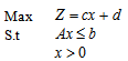Where is a constant term in the objective function.

To solve such problem, we keep the constant term aside and apply the appropriate method of solving the LP. When the Objective function is determined, we then add the constant term to objective function to obtain the required optimal objective Function.

3.2. Revised Simplex Method (RSM)

Original simplex method calculates and stores all numbers in the tableau. Revised Simplex Method which is more efficient for computing Linear programming problems operates on a data structure that is roughly of size m by m instead of the whole tableau.

Initially constraints become the standard form:

Where slack variables

Basis matrix: columns relating to basic variables.

(Initially B=I )

Basic variable values:

At any iteration non-basic variables =0

Where is the inverse matrix

At any iteration, given the original vector and the inverse matrix, (current R.H.S.) can be calculated.

Where = objective coefficients of basic variables.

3.2.1. Steps in the Revised Simplex Method

1. Determine entering variable, , with associated vector .

Compute

Compute for all non-basic variables.

Choose largest negative value (maximization).

If none, stop.

2. Determine leaving variable, , with associated vector P_r.

Compute (current R.H.S.)

Compute current constraint coefficients of entering variable:

is associated with

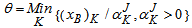i.e. minimum ratio rule

3. Determine next basis i.e. calculate .

Go to step 1.

Example:

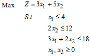
First Iteration

Step 1

Determine entering variable, , with associated vector .

Compute

Compute for all non-basic variables (

and similarly for Z₂– c₂= - 5

Therefore X₂ is entering variable.

Step 2

Determine leaving variable, , with associated vector P_r.

Compute = B^-1b (current R.H.S.)

Compute current constraint coefficients of entering variable:

is associated with

Therefore S₂ leaves the basis.

Step 3

Determine new

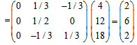
Solution after one iteration:

= B^-1b =

Go to step 1

Second Iteration

Step 1

Compute

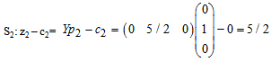
Compute for all non-basic variables ( and S₂):-

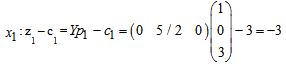
Therefore enters the basis.

Step 2

Determine leaving variable.

θ = Min { 4/1 , - , 6/3 }

= 6/3

Therefore S₃ leaves the basis.

Step 3

Determine new

Solution after two iterations:

Go to step 1

Third Iteration

Step 1

Compute

Compute for all non-basic variables (S₂ and S₃):-

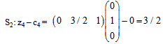
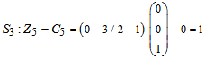No negatives. Therefore stop.

Optimal solution:

S₁* = 2

X₂* = 6

X₁* = 2

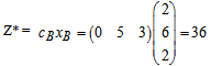Therefore, the Optimal objective function is 36 where 2 and .

3.3. Sensitivity Analysis

Sensitivity analysis helps to determine the effect of changes in the parameters of the Linear Programming model in other to determine the optimal solution. That is, it allows the analyst to determine the behaviour of the optimal solution as a result of making changes in the model’s parameters.

3.3.1. Changing Objective Function

Consider the LPP below.

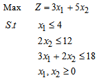Suppose in the solution of the LPP above, we wish to solve another problem with the same constraints but a slightly different objective function. So if the objective function is changed, not only will I hold the constraints fixed, but I will change only one coefficient in the objective function. When you change the objective function it turns out that there are two cases to consider. The first case is the change in a non-basic variable (a variable that takes on the value zero in the solution). In the example, the relevant non-basic variables are and . What happens to your solution if the coefficient of a non-basic variable decreases? For example, suppose that the coefficient of in the objective function above was reduced from 3 to 2 (so that the objective function is: ). What has happened is this: You have taken a variable that you didn’t want to use in the first place (i.e. you set = 0) and then made it less profitable (lowered its coefficient in the objective function). You are still not going to use it. The solution does not change.

Observation: If you lower the objective function coefficient of a non-basic variable, then the solution does not change. What if you raise the coefficient? Intuitively, raising it just a little bit should not matter, but raising the coefficient a lot might induce you to change the value of in a way that makes > 0. So, for a non-basic variable, you should expect a solution to continue to be valid for a range of values for coefficients of non-basic variables. The range should include all lower values for the coefficient and some higher values. If the coefficient increases enough and putting the variable into the basis is feasible, then the solution changes.

What happens to your solution if the coefficient of a basic variable (like in the example) decreases? The change makes the variable contribute less to profit. You should expect that a sufficiently large reduction makes you want to change your solution. For example, if the coefficient of in the objective function in the example was 2 instead of 5 (so that the objective was ), will change the solution since the reduction in the coefficient of is large. On the other hand, a small reduction in objective function coefficient would typically not cause you to change your solution.

So, intuitively, there should be a range of values of the coefficient of the objective function (a range that includes the original value) in which the solution of the problem does not change. Outside of this range, the solution will change. The value of the problem always changes when you change the coefficient of a basic variable.

3.3.2. Changing a Right-Hand Side Constant of Constraint

When you changed the amount of resource in a non-binding constraint, i.e. small increases will never change your solution and small decreases will also not change anything. However, if you decreased the amount of resource enough to make the constraint binding, your solution could change. But, changes in the right-hand side (RHS) of binding constraints always change the solution.

3.3.3. Adding a Constraint

If you add a constraint to a problem, two things can happen. Your original solution satisfies the constraint or it doesn’t. If it does, then you are finished. If you had a solution before and the solution is still feasible for the new problem, then you must still have a solution. If the original solution does not satisfy the new constraint, then possibly the new problem is infeasible. If not, then there is another solution.

4. Results and Discussions

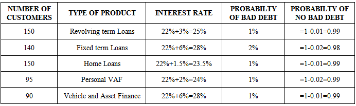
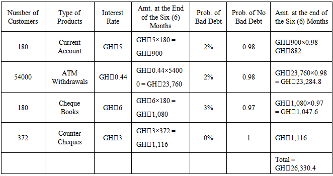
The research was a case paper of Bank X Tamale-Ghana. The data type is secondary data in the areas of interest from loans such as Revolving Term Loans, Fixed Term Loans, Home Loans, Personal VAF, Vehicle and Asset Finance as well as interest derived from Current Accounts, ATM withdrawals, Cheque Books and Counter Cheques of at least 90 customers for the period of six (6) months from November, 2011 to April, 2012 as shown in table 4.1 and 4.2.

Table 4.1. Data of Bank X for the Period of Six (6) Months (Nov. 2011 to April, 2012) of Variable Products (i.e. Loans)

Table 4.2. Data of Bank X for the Period of Six (6) Months (Nov. 2011 to April, 2012) of Constant Products

The bank is to allocate a total fund of GH₵3,745,200 to the various loan products. The bank is faced with following constraints:

Amounts allocated to the various loan products should not be more than the total funds.

Allocate not more than 60% of the total funds to Fixed term loans, Personal VAF; and Vehicle and Asset loans.

Revolving term loans, Fixed term loans and Personal VAF should not be more than 50% of the total funds.

Allocate not more than 40% of the total funds to Personal VAF and Vehicle and Asset loans.

The overall bad debts on the Revolving term loans, Fixed term loans, Home loans, Personal VAF; and Vehicle and Asset Loans should not exceed 0.03 of the total funds.

4.1. Mathematical Model

The variables of the model are defined as

= Revolving term loans (in millions in GH₵)

= Fixed term loans

= Home loans

= Personal VAF

= Vehicle and Asset finance

The objective of Bank X Tamale was to maximize its net returns consisting of the difference between the revenue from interest and lost funds due to bad debts.

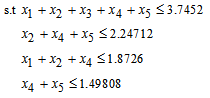
The problem has six (6) constraints:

Total funds:

Allocate not more than 60% of the total funds to Fixed term loans, Personal VAF; and Vehicle and Asset loans:

Revolving term loans, Fixed term loans and Personal VAF should not be more than 50% of the total funds:

Allocate not more than 40% of the total funds to Personal VAF and Vehicle and Asset loans:

The overall bad debts on the Revolving term loans, Fixed term loans, Home loans, Personal VAF; and Vehicle and Asset Loans should not exceed 0.03 of the total funds:

Non-negativity constraint:

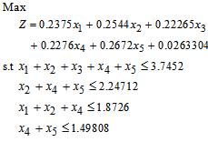
Now the LP is

Max

s.t

4.2. Using the Revised Simplex Method to Solve the Lpm

The Linear Programming Model (LPM) of the problem of Profit Optimization of Bank X Tamale-Ghana was

Max

Standard form of constraints is:

FIRST ITERATION

Step 1

Determine entering variable, , with associated vector .

Compute

Compute for all non-basic variables.

Similarly for

Z₃ – c₃ = - 0.22265

Z₄ – c₄ = - 0.2276

Z₅ – c₅ = - 0.2672

Therefore X₅ is entering variable.

Step 2

Determine leaving variable, , with associated vector

Compute (current RHS)

Compute current constraint coefficients of entering variable

is associated with

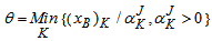
Therefore S₄ leaves the basis.

Step 3

Determine new

Solution after one iteration:

Go to step 1

SECOND ITERATION

Step 1

Determine entering variable, , with associated vector .

Compute

Compute 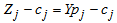for all non-basic variables

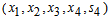
Therefore X₂ is entering variable.

Step 2

Determine leaving variable, , with associated vector

Compute (current RHS)

Compute current constraint coefficients of entering variable

is associated with

Therefore S₂ leaves the basis.

Step 3

Determine new

Solution after two iterations:

Go to step 1

THIIRD ITERATION

Step 1

Determine entering variable, , with associated vector .

Compute

Compute for all non-basic variables

Therefore X₁ is entering variable.

Step 2

Determine leaving variable, , with associated vector

Compute (current RHS)

Compute current constraint coefficients of entering variable

is associated with

Therefore S₃ leaves the basis.

Step 3

Determine new

Solution after three iterations:

Go to step 1

FOUTH ITERATION

Step 1

Determine entering variable, , with associated vector .

Compute

Compute for all non-basic variables

Therefore X₃ is enters the basis.

Step 2

Determine leaving variable, , with associated vector

Compute (current RHS)

Compute current constraint coefficients of entering variable

is associated with

Therefore S₁ leaves the basis.

Step 3

Determine new

Solution after four iterations:

Go to step 1

FIFTH ITERATION

Step 1

Determine entering variable, , with associated vector .

Compute

Compute for all non-basic variables

No negatives. Therefore, stop.

Optimal Solution:

The optimum objective function value= 0.9410751 (in millions GH₵).

The optimum solution is:

= 1.123560 (in millions)

= 0. 7490400

= 0. 3745200

= 0

= 1.498080

However, the objective function in the LPP was having a constant term of 0.0263304 which was then added to the optimum objective function value of 0.9410751 to obtain an Optimal Profit of GH₵0.9674055 (in millions). i.e. the Optimal Profit of Bank X Tamale in the areas of interest from loans such as Revolving Term Loans, Fixed Term Loans, Home Loans, Personal VAF, Vehicle and Asset Finance as well as interest derived from Current Accounts, ATM withdrawals, Cheque Books and Counter Cheques of at least 90 customers for the period of six (6) months from November, 2011 to April, 2012 was GH₵967,405.5

Therefore, for the bank to achieve the Optimal Profit of GH₵967,405.5, Revolving Term Loans must be allocated an amount of GH₵1,123,560; Fixed Term Loans an amount of GH₵749,040; Home Loans an amount of GH₵374,520; Personal VAF an amount of GH₵0.00; Vehicle and Asset Finance an amount of GH₵1,498,080.

4.3. Sensitivity Analysis

In the linear programming model of the data of Bank X Tamale, we may want to see how the answer changes if the problem is changed. In every case, the results assume that only one thing about the problem changes. That is, in sensitivity analysis you evaluate what happens when only one parameter of the problem changes.

The solution to this problem was:

= 1.123560 (in millions)

= 0. 7490400

= 0. 3745200

= 0

= 1.498080

4.3.1. Changing Objective Function

Suppose in the solution of the LPP above, we wish to solve another problem with the same constraints but a slightly different objective function. When you change the objective function it turns out that there are two cases to consider. The first case is the change in a non-basic variable (a variable that takes on the value zero in the solution). In the LPP above, the relevant non-basic variables are . What happens to your solution if the coefficient of a non-basic variable decreases? For example, suppose that the coefficient of in the objective function above was reduced from 0.2375 to 0.11 so that the objective function is:

Max

What has happened is this: You have taken a variable that you didn’t want to use in the first place (i.e. you set = 0) and then made it less profitable (lowered its coefficient in the objective function). You are still not going to use it. The solution does not change.

Observation: If you lower the objective function coefficient of a non-basic variable, then the solution does not change. What if you raise the coefficient? Intuitively, raising it just a little bit should not matter, but raising the coefficient a lot might induce you to change the value of in a way that makes > 0. So, for a non-basic variable, you should expect a solution to continue to be valid for a range of values for coefficients of non-basic variables. The range should include all lower values for the coefficient and some higher values. If the coefficient increases enough and putting the variable into the basis is feasible, then the solution changes.

What happens to your solution if the coefficient of a basic variable (like in the LPP) decreases? The change makes the variable contribute less to profit. You should expect that a sufficiently large reduction makes you want to change your solution. For example, if the coefficient of in the objective function in the example was 0.1411 instead of 0.2672 (so that the objective was ), will change the solution since the reduction in the coefficient of is large. On the other hand, a small reduction in objective function coefficient would typically not cause you to change your solution.

So, intuitively, there should be a range of values of the coefficient of the objective function (a range that includes the original value) in which the solution of the problem does not change. Outside of this range, the solution will change. The value of the problem always changes when you change the coefficient of a basic variable.

4.3.2. Changing a Right-Hand Side (RHS) Constant of a Constraint

When you changed the amount of resource in a non-binding constraint, i.e. small increases will never change your solution and small decreases will also not change anything. However, if you decreased the amount of resource enough to make the constraint binding, your solution could change. But, changes in the right-hand side of binding constraints always change the solution.

4.3.3. Adding a Constraint

If you add a constraint to a problem, two things can happen. Your original solution satisfies the constraint or it doesn’t. If it does, then you are done. If you had a solution before and the solution is still feasible for the new problem, then you must still have a solution. If the original solution does not satisfy the new constraint, then possibly the new problem is infeasible. If not, then there is another solution.

5. Conclusions

Based on the results of our analysis, it can be concluded that Profit Optimization in Bank X Tamale-Ghana can be achieved through LP modeling of the problem and using the Revised Simplex Method to solve the LP. It was realized that the Optimal Profit of Bank X Tamale-Ghana in areas of interest from loans such as Revolving Term Loans, Fixed Term Loans, Home Loans, Personal VAF, Vehicle and asset Finance as well as interest derived from Current Accounts, ATM withdrawals, Cheque Books and Counter Cheques of at least 90 customers for the period of six (6) months from November, 2011 to April, 2012 was GH₵967,405.5.

Therefore, for the bank to achieve the Optimal Profit of GH₵967,405.5, Revolving Term Loans must be allocated an amount of GH₵1,123,560; Fixed Term Loans an amount of GH₵749,040; Home Loans an amount of GH₵374,520; Personal VAF an amount of GH₵0.00; Vehicle and Asset Finance an amount of GH₵1,498,080.

It was also observed that if Bank X Tamale-Ghana does not allocate any amount to Personal VAF, the bank can still achieve the Optimal Profit of GH₵967,405.50

Finally, by comparing the amounts allocated to each product, the bank should allocate more amounts to Vehicle and Asset Finance, Revolving Term Loans and Fixed Term Loans if the bank desires to achieve the Optimal profit of GH₵967,405.50