Rasi Muthuramalingam, Vembu Ananthaswamy, Rajendran Lakshmanan
Department of Mathematics, The Madura College, Madurai, India
Correspondence to: Rajendran Lakshmanan, Department of Mathematics, The Madura College, Madurai, India.
| Email: |  |
Copyright © 2014 Scientific & Academic Publishing. All Rights Reserved.
Abstract
In this paper, a mathematical modelling of cholera epidemics is discussed. Approximate analytical solutions for the non-linear equations in cholera epidemics are obtained by using the Homotopy analysis method (HAM). Analytical expressions pertaining to the number of susceptible, infected individuals, concentration of Vibrio cholera and recovered individuals have been derived for all possible values of parameters. Furthermore, in this work the numerical simulation of the problem is also reported using Matlab program to investigate the dynamics of the system. Graphical results are presented and discussed quantitatively to illustrate the solution. A satisfactory agreement between analytical and numerical results is noted.
Keywords:
Cholera epidemics, Mathematical modelling, Homotopy analysis method, Nonlinear differential equations
Cite this paper: Rasi Muthuramalingam, Vembu Ananthaswamy, Rajendran Lakshmanan, Nonlinear Analysis of Cholera Epidemics, Applied Mathematics, Vol. 4 No. 1, 2014, pp. 12-21. doi: 10.5923/j.am.20140401.02.
1. Introduction
Cholera is an intestinal disease caused by the bacterium Vibrio cholera, which colonizes the human intestine. Transmission occurs primarily by drinking water or eating food that has been contaminated by the waste product of an infected person, including one with no apparent symptoms. The infection can spread from inland regions with epidemic outbursts into the surrounding areas. In fact, cholera still represents a global threat to public health [4], especially in developing countries where infrastructures to provide access to safe water and basic sanitation are lacking. Spatial and temporal patterns of cholera epidemics are strongly related to the ecology of the bacterium in the environment driven by hydrological and climatic variability. An important determinant of the disease spatial-temporal variability is the environmental matrix in which the disease spreads into disease-free regions. The matrix is constituted by different human communities and their hydrological inter connections. Each community is characterized by its spatial position, population size, water resource availability and hygiene conditions. Bertuzzo et al. [1] generalize the models of cholera epidemics that accounts for local communities of susceptible and infective in a spatially explicit arrangement. The mathematical tools used here is the general schemes of reactive transport on river networks acting as the environmental matrix for the circulation and mixing of waterborne pathogens. Mathematical models of infectious diseases can provide important insight into our understanding of epidemiological processes, the course of infection within a host, the transmission dynamics in a host population, and implementation of infection control programs [15].Several studies suggest that the number of susceptible, exposure to untreated water and the presence of Vibrio cholera in the aquatic environment are the important factors to understand the cholera epidemics [5-8]. The purpose of this paper is to provide approximate analytical expressions for the number of susceptible, infective, concentration of Vibrio cholera and recovered individuals. We also investigate the influence of parameters like net growth rate, rate of exposure to contaminated water and contribution of each infected person to the population of Vibrio cholera in the aquatic environment.
2. Mathematical Formulation
In this paper, the mathematical model of the susceptible, infected and recovered class with a reservoir of free-living pathogens is used. It is an extension of the (SIB) cholera epidemic model introduced by Codeço [2]. The SIB model is a standard compartmental model that has been used to describe many epidemiological diseases [7, 14, 18, 20]. The local epidemic model has state variables, namely the number of susceptible (S) and infected individuals (I) in a human community of size H, concentration of Vibrio cholerae (B) in the aquatic environment and the recovered individuals (R). The temporal evolution of state variables can be described by the following system of nonlinear differential equations [1]. | (1) |
 | (2) |
 | (3) |
 | (4) |
Equation (1) describes the dynamics of susceptible in a human population of size  . Susceptible individuals are born and die on average at rate
  . Rate of susceptible individuals is directly proportional to
  . Newborn individuals are considered susceptible. A susceptible individual will move into the infected group through contact with an infected individual, approximated by an average contact rate
  , where
  is the rate of contact with contaminated water and
  is the probability of such person to catch cholera and
  is the semi saturation concentration [2]. Probability of catching cholera depends on the concentration of Vibrio cholera in the consumed water. Second equation describes the dynamics of infected with the recovery rate
  and disease-induced mortality rate
  . The third equation expresses the dynamics of the free-living infective agents in the aquatic reservoir. Infected people contribute to the concentration of vibrios at a rate
  , where
  is the rate at which bacteria produced by one infected person and
  is the volume of water reservoir.
  represents the growth rate of Vibrio cholera in the aquatic environment. The fourth equation defines the recovery rate. People recovered from cholera are considered immune.As long as we are not interested in the numerical value, we can introduce the new parameters
  which are normalized and
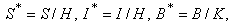

 where
where  is the rate at which people recover from cholera and
  is the contribution of each infected person to the population of Vibrio cholerae (B) in the aquatic environment. The governing differential equations for cholera epidemic model in one dimension with initial conditions are as follows:
 | (5) |
 | (6) |
 | (7) |
 | (8) |
 | (9) |
The model predicts an epidemic outbreak under the above initial condition only if the reproduction number  or
or  .
.
3. Analytical Solutions of Number of Susceptible, Infected Individuals, Concentrations of Vibrio Cholera and People Recovered from Cholera Using the Homotopy Analysis Method
Liao [9, 11] proposed a powerful analytical method for solving the nonlinear problems, namely the Homotopy analysis method (see Appendix A). Different from all perturbation and non-perturbative techniques, the Homotopy analysis method [3, 12, 16, 21] itself provides us with a convenient way to control and adjust the convergences region and rate of approximation series, when necessary. The Homotopy analysis method has the following advantages: It is valid even if a given nonlinear problem does not contain any small/large parameters at all; it can be employed to efficiently approximate a nonlinear problem by choosing different sets of base functions. The Homotopy analysis method is an extremely simple method [10] to solve the non-linear differential equations. Furthermore, the obtained result is of high accuracy. Using this Homotopy analysis method (see Appendix B), we obtained the analytical expression corresponding to susceptible, infected individuals, concentrations of Vibrio cholera and people recovered from cholera as follows: | (10) |
 | (11) |
 | (12) |
 | (13) |
4. Numerical Simulation
In order to investigate the accuracy of the analytical solution with a finite number of terms, the system of differential equations were solved numerically. To show the efficiency of the present method our results are compared with the numerical solution (MATLAB program). The function ode45 (Range-Kutta method) in Matlab software [19] which is a function of solving the initial value problems is used to solve Eqns. (5) – (8). The analytical solution of number of susceptible, infected individuals, concentrations of Vibrio cholera and people recovered from cholera are compared with the numerical solution in Figs. (1) to (8). The average relative error between our analytical work and numerical result for susceptible is 0%, 0.001%, and 0.008% when θ = 0.05, 1 and 2 respectively. The Matlab program [17] is also given in Appendix C.
5. Discussion
Eqns. (10) - (13) represents the new and simple analytical expressions for the number of susceptible, infected individuals, concentration of Vibrio cholera and people recovered from cholera respectively. In order to analyse the influence of parameters like  (Natality and mortality rates of susceptible),
  (Rate of exposure to contaminated water),
  (Rate at which people recover from Cholera),
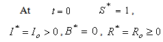
  (Mortality rate due to Cholera) etc., over cholera epidemics, the analytical expressions (Eqns. (10) – (13)) are plotted in Fig. (1) – Fig. (5). Fig. 1 and 2 represents the profile of susceptible individuals
  versus time t for various values of
  and
and  respectively and for some fixed values of the parameters


 . From Fig. 1(a) it is observed that the number of susceptible decreases when contribution of each infected person to the population of Vibrio cholera (B) in the aquatic environment
 increases. Fig. 1(b) proves that, when the rate of exposure to contaminated water
  and time t increases the susceptible level decreases. Hence, from the figures 1(a) and 1(b) it is evident that to protect the susceptible from infection we have to minimize the rate of
  and
and  .
. | Figure 1(a). Number of susceptible  versus time t for various values of versus time t for various values of  is plotted using Eqn. (10). The key to the graph: solid line represents the Eqn. (10) and dotted line represents the numerical simulation is plotted using Eqn. (10). The key to the graph: solid line represents the Eqn. (10) and dotted line represents the numerical simulation |
 | Figure 1(b). Number of susceptible  versus time t for various values of versus time t for various values of  is plotted using Eqn. (10). The key to the graph: solid line represents the Eqn. (10) and dotted line represents the numerical simulation is plotted using Eqn. (10). The key to the graph: solid line represents the Eqn. (10) and dotted line represents the numerical simulation |
Fig. 2(a) and 2(b) represents the profile of Infected individuals  versus time t for various values of parameters. From Fig. 2(a), it is evident that the infected rate increases with increasing the rate of
  . But when the time increases it gradually decreases and reaches the steady state. From Fig. 2(b), it is inferred that the number of infected decreases when
  increases. From these figures we conclude that even if the rate of
  and
and  increases, the infected rate
  decreases after some period of time. Fig. 3(a) and 3(b) represents the concentration of Vibrio cholera
  versus time t for various values of parameters. In Fig. 3(a), it is seen that the concentration of Vibrio cholera remains constant when
  is small. And when the value of
  increases the concentration of cholera increases. After some period of time (
 day), the concentration of cholera
  starts decreasing and it reaches the steady state value when
  . Hence for our fixed value of
  the bacteria Vibrio cholera is active only up to the day 5 and after the 5th day it loses its power. From Fig. 3(b), we confirm that decreasing the value of
  increases the concentration of Vibrio cholera. For
  = 0.02, the concentration starts decreases when
  day. And for
  = 0.37, it starts decreasing when
  . Therefore comparing the parameters
  and
and  ,
,  affect the concentration of cholera more than
  . Fig. 4(a) and 4(b) represents the number of recovered people
  versus time t for various values of parameters. From Fig. 4(a), it is obvious when the recovery rate
  is small the number of people recovered from cholera
  remains constant or unique. Similarly from Fig. 4(b), it is seen that to increase the recovery rate we have to decrease the natality and mortality rate
  .
.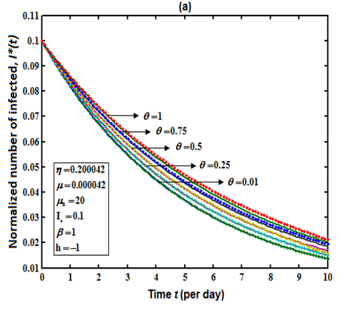 | Figure 2(a). Number of infected  versus time t for various values of is plotted using Eqn. (11). The key to the graph: solid line represents the Eqn. (11) and dotted line represents the numerical simulation versus time t for various values of is plotted using Eqn. (11). The key to the graph: solid line represents the Eqn. (11) and dotted line represents the numerical simulation |
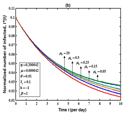 | Figure 2(b). Number of infected  versus time t for various values of versus time t for various values of  is plotted using Eqn. (11). The key to the graph: solid line represents the Eqn. (11) and dotted line represents the numerical simulation is plotted using Eqn. (11). The key to the graph: solid line represents the Eqn. (11) and dotted line represents the numerical simulation |
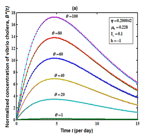 | Figure 3(a). Concentration of Vibrio cholera  versus time t for various values of versus time t for various values of  is plotted using Eqn. (12). The key to the graph: solid line represents the Eqn. (12) and dotted line represents the numerical simulation is plotted using Eqn. (12). The key to the graph: solid line represents the Eqn. (12) and dotted line represents the numerical simulation |
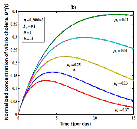 | Figure 3(b). Concentration of Vibrio cholera  versus time t for various values of death rate versus time t for various values of death rate  is plotted using Eq. (12). The key to the graph: solid line represents the Eq. (12) and dotted line represents the numerical simulation is plotted using Eq. (12). The key to the graph: solid line represents the Eq. (12) and dotted line represents the numerical simulation |
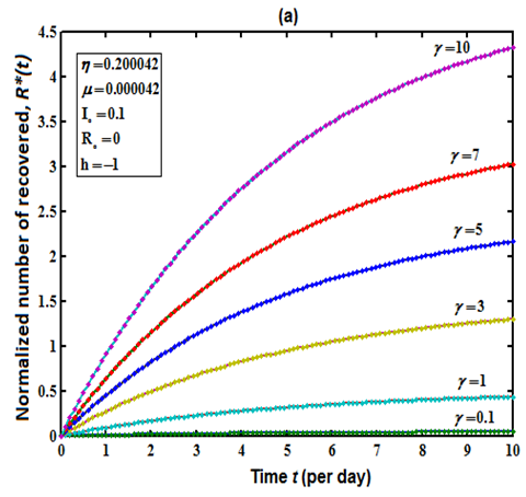 | Figure 4(a). Number of recovered  versus time t for various values of versus time t for various values of  is plotted using Eqn. (13). The key to the graph: solid line represents the Eqn. (13) and dotted line represents the numerical simulation is plotted using Eqn. (13). The key to the graph: solid line represents the Eqn. (13) and dotted line represents the numerical simulation |
 | Figure 4(b). Number of recovered  versus time t for various values of versus time t for various values of  and and  is plotted using Eqn. (13). The key to the graph: solid line represents the Eqn. (13) and dotted line represents the numerical simulation is plotted using Eqn. (13). The key to the graph: solid line represents the Eqn. (13) and dotted line represents the numerical simulation |
The population of susceptibles  , infected individuals
  , concentration of Vibrio cholera
  and number of people recovered from cholera
  are plotted together for particular values of the parameters in Fig. 5. From this figure, we confirm that as the infected individuals and concentration of bacteria increases the susceptible rate decreases with respect to time t. For large values of t the rate of susceptible and infected reaches the steady state but the concentration of Bacteria decreases. Compared to the population of others, the population of recovered increases with time and after some values of t it remains constant. Table 1 represents the comparison of analytical result with the numerical result of susceptible
  for various values of
  and for some fixed values of when
  and
and  using Eqn. (10). From this table, it is inferred that the rate of susceptible
  decreases when
  increases. By setting the derivatives of Eqns. (5) – (8) to zero and solving it algebraically, the equilibrium (or steady state) values can be obtained as follows:
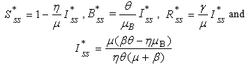 | (14) |
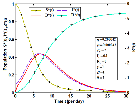 | Figure 5. Population of susceptible , infected , infected , recovered , recovered  and concentration of Vibrio cholera and concentration of Vibrio cholera  versus time t is plotted using Eqns. (10) to (13) versus time t is plotted using Eqns. (10) to (13) |
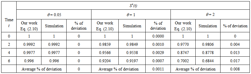 | Table 1. Comparison of analytical result with the numerical result of susceptible  for various values of for various values of  and for some fixed values of and for some fixed values of  using Eq. (10) using Eq. (10) |
The above equilibrium values are positive only if  or
or  . The limitation condition of proposed solution for the model system is
  | (15) |
Under this condition, the proposed model is feasible.
6. Conclusions
Time dependent non-linear differential equations in cholera epidemic models have been solved analytically. The model investigated the influence of parameters over cholera with respect to time (days). Approximate analytical expressions pertaining to the number of susceptible, infected individuals, concentration of Vibrio cholera and people recovered from cholera for all values of the parameters are obtained using the Homotopy analysis method. Using this result, it is possible to predict the crucial stage to control the growth of Vibrio which lends a hand to decrease the rate of infected and to increase the rate of recovered. This analytical result helps us for the better understanding of Vibrio ecology and epidemiology.
Appendix A
Basic concepts of Liao’s Homotopy analysis methodConsider the following differential equation [10]: | (A1) |
where Ν is a nonlinear operator, x denotes an independent variable, u(x) is an unknown function. For simplicity, we ignore all boundary or initial conditions, which can be treated in the similar way. By means of generalizing the conventional homotopy method [12], constructed the so-called zero-order deformation equation as: | (A2) |
where p [0,1] is the embedding parameter, h ≠ 0 is a nonzero auxiliary parameter, H(x) ≠ 0 is an auxiliary function, L is an auxiliary linear operator,
  (x) is an initial guess of u(x),
  is an unknown function. It is important, that one has great freedom to choose auxiliary unknowns in HAM. Obviously, when
  and
and , it holds:
 | (A3) |
respectively. Thus, as p increases from 0 to 1, the solution  varies from the initial guess
  to the solution u (x). Expanding
  in Taylor series with respect to p, we have:
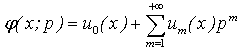 | (A4) |
where 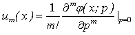 | (A5) |
If the auxiliary linear operator, the initial guess, the auxiliary parameter h, and the auxiliary function are so properly chosen, the series (A4) converges at p =1 then we have: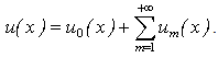 | (A6) |
 | (A7) |
Differentiating Eq. (A2) for m times with respect to the embedding parameter p, and then setting p = 0 and finally dividing them by m!, we will have the so-called mth-order deformation equation as: | (A8) |
where  | (A9) |
and | (A10) |
Applying  on both side of equation (A8), we get
 | (A11) |
In this way, it is easily to obtain  for
for  at
at  order, we have
 When
When  , we get an accurate approximation of the original equation (A1). For the convergence of the above method we refer the reader to [10]. If equation (A1) admits unique solution, then this method will produce the unique solution. If equation (A1) does not possess unique solution, the HAM will give a solution among many other (possible) solutions.
Appendix B
Approximate analytical solutions for Eqns. (5) - (8) using the HAMIn order to solve eqns. (5) - (8) by means of the HAM, we first construct the Zeroth order deformation equation by taking  .
.  | (B1) |
 | (B2) |
 | (B3) |
 | (B4) |
The approximate solutions of eqns. (B1), (B2), (B3) and (B4) are as follows  | (B5) |
 | (B6) |
 | (B7) |
 | (B8) |
Substituting (B5) and (B7) in eqn. (B1) and equating the like powers of p we get  | (B9) |
 | (B10) |
 | (B11) |
Substituting (B5) – (B7) in eqn. (B2) and equating the like powers of p we get  | (B12) |
 | (B13) |
 | (B14) |
Substituting (B6) and (B7) in eqn. (B3) and equating the like powers of p we get  | (B15) |
 | (B16) |
 | (B17) |
Substituting (B6) and (B8) in eqn. (B4) and equating the like powers of p we get  | (B18) |
 | (B19) |
 | (B20) |
The boundary conditions in eqn. (9) becomes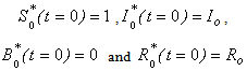 | (B21) |
and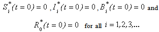 | (B22) |
Now applying the boundary conditions (B21) in (B5) and (B7) we get  | (B23) |
 | (B24) |
 | (B25) |
 | (B26) |
Substituting the values of 
 ,
,  and
and  in Eqn. (B10), (B13), (B16) and (B19) and solving the equations using the boundary conditions (B22) we obtain the following results:
 | (B27) |
 | (B28) |
 | (B29) |
 | (B30) |
Substituting the values of 


 ,
, ,
, ,
, and
and  in eqn. (B11), (B14), (B17) and (B20) and solving the equations using the boundary conditions (B22) we obtain the following results:
 | (B31) |
 | (B32) |
 | (B33) |
 | (B34) |
Substituting eqns. (B23) to (B34) in eqns. (B5) to (B8), we get the solutions as follows | (B35) |
 | (B36) |
 | (B37) |
 | (B38) |
The analytical solution represented by the eqns. (B35) to (B38) contains the auxiliary parameter  which gives the convergence region and the rate of approximation for HAM. The auxiliary parameter
  controls the convergence and accuracy of the solution series [13]. The parameter
  is chosen as
  throughout this paper to show the accuracy of the solution and it gives better results.
Appendix C
Scilab/Matlap program for the numerical solution of the system of non-linear differential Eqns. (5) – (8).function graphmain3options= odeset('RelTol',1e-6,'Stats','on');%initial conditionsXo = [1; 0.1; 0]; tspan = [0 1]; tic[t,X]=ode45(@TestFunction,tspan,Xo,options);toc figurehold onplot(t, X(:,1),'-')%plot(t, X(:,2),'-')%plot(t, X(:,3),'-')legend('x1','x2','x3')ylabel('x')xlabel('t') return function [dx_dt]= TestFunction(t, x)e=4.2*10^(-5);c1=1;c2=0.2+4.2*10^(-5);c3=0.228;c4=0.05; dx_dt(1) = e*(1-x(1))-c1*x(1)*x(3)/(1+x(3));dx_dt(2) = c1*x(1)*x(3)/(1+x(3))-c2*x(2); dx_dt(3) =-c3*x(3)+c4*x(2);dx_dt = dx_dt'; return
Appendix D
NomenclatureState variablesS Number of susceptibleI Number of infected B Concentration of Vibrio cholera in aquatic environment (Cells/m-3)R Number of recoveredParametersH Total human population sizeK Concentration of Vibrio cholera in water that yields 50% chance of being infected with cholera (Cells/m-3) and mortality rates of susceptible (per day)
  of exposure to contaminated water (per day)
  at which people recover from cholera (per day)
 rate due to cholera (per day)
 growth rate of Vibrio cholera in the aquatic environment (per day)
 of production by one person infected of Vibrio cholera that reach the water body (Cells/m-3 per day per person)
 (per day)New parametersS* Normalized number of susceptibleI* Normalized number of infected B* Normalized concentration of Vibrio cholera in aquatic environment R* Normalized number of recovered
 at which people recover from cholera (per day)
 of each infected person to the population of Vibrio cholerae (B) in the aquatic environment (per day per person)
 Reproduction number
References
| [1] | E. Bertuzzo, R. Casagrandi, M. Gatto, I. Rodriguez-Iturbe, A. Rinaldo, On spatially explicit models of cholera epidemics. J R Soc Interface (2009). |
| [2] | C. Codec¸o, Endemic and epidemic dynamics of cholera: the role of the aquatic reservoir. BMC Infect Dis 1(2001), 1. |
| [3] | G. Domairry, M. Fazeli, Homotopy analysis method to determine the fin efficiency of convective straight fins with temperature-dependent thermal conductivity. Commun Nonlinear Sci Numer Simul 14(2009),489– 499. |
| [4] | M. Emch, C. Feldacker, M. S. Islam, M. Ali, Seasonality of cholera from 1974 to 2005: a review of global patterns. Int J Health Geogr 7(2008), 31. |
| [5] | P. R. Epstein, Algal blooms in the spread and persistence of cholera. Biosystems 31(1993), 209-221. |
| [6] | S. M. Faruque, M. J. Albert, J. Mekalanos, Epidemiology, genetics and ecology of toxigenic Vibrio cholera. Microbiology and Molecular Biology Reviews 62(1998), 1301-1314. |
| [7] | H. W. Hethcote, The mathematics of infectious diseases. Siam Rev 42(2000), 599–653. |
| [8] | M. S. Islam, B. Drasar, S. R. Bradley, Probable role of blue-green algae in maintaining endemicity and seasonality of cholera in Bangladesh: a hypothesis. J Diarrhoeal Dis Res 12(1994), 245-256. |
| [9] | S. J. Liao, Proposed homotopy analysis techniques for the solution of nonlinear problems. Dissertation, Shanghai Jiaotong University (1992). |
| [10] | S. J. Liao Beyond Perturbation: Introduction to the Homotopy analysis method. 1st Edn. Chapman and Hall, CRC Press, Boca Raton (2003). |
| [11] | S. J. Liao, Y. Tan, A general approach to obtain series solutions of nonlinear differential equations. Studies in Applied Mathematics 119(2007), 297-354. |
| [12] | S. J. Liao, An optimal homotopy-analysis approach for strongly nonlinear differential equations. Comm Nonlinear Sci Numer Simulat 15(2010), 2003-2016. |
| [13] | S. J. Liao, Homotopy analysis method in Nonlinear Differential Equations. Springer: Berlin, Germany (2012). |
| [14] | Z. Lu, X. Chi, L. Chen, The effect of constant and pulse vaccination of SIR epidemic model with horizontal and vertical transmission. Math Comput Model 36(2002), 1039–1057. |
| [15] | Madan K. Oli, Meenakshi Venkataramana, Paul A. Kleinb, Lori D. Wendlandc, Mary B. Brownc, Population dynamics of infectious diseases: A discrete time model. Ecological modelling 198(2006), 183–194. |
| [16] | A. Mastroberardino, Homotopy Analysis Method Applied to Electrohydrodynamic Flow. Comm Nonlinear Sci Numer Simulat 16(2010), 2730 -2736. |
| [17] | MATLAB 6.1, The MathWorks Inc., Natick, MA, 2000. |
| [18] | C. Piccolo III, L. Billings, The effect of vaccinations in an immigrant model. Math Comput Model 42(2005), 291–299. |
| [19] | R. D. Skeel, M. Berzins, A Method for the Spatial Discretization of Parabolic Equations in One Space Variable. SIAM Journal on Scientific and Statistical Computing 11(1990), 1-32. |
| [20] | H. L. Smith, Subharmonic bifurcation in SIR epidemic model. J Math Biol 17(1983) ,163–177. |
| [21] | A. R. Sohouli, M. Famouri, A. Kimiaeifar, G. Domairry, Application of homotopy analysis method for natural convection of Darcian fluid about a vertical full cone embedded in porus media prescribed surface heat flux.Comm Nonlinear Sci Numer Simulat 15(2010), 1691-1699. |
 Abstract
 Reference
 Full-Text PDF
 Full-text HTML