Quang Phung Duy
Department of Mathematics, Foreign Trade University, Ha noi, Viet Nam
Correspondence to: Quang Phung Duy , Department of Mathematics, Foreign Trade University, Ha noi, Viet Nam.
| Email: |  |
Copyright © 2012 Scientific & Academic Publishing. All Rights Reserved.
Abstract
The aim of this paper is to give recursive and integral equations for ruin probabilities of generalized risk processes under assumption that both sequences of claims and rates of interest are homogenous Markov chains. Generalized Lundberg inequalities for ruin probabilities of these processes are derived by using recursive technique. Firstly, we give a recursive equations for finite – time probability and ultimate ruin probability. By using these equations, we can derive probability inequalities for finite – time probability and ultimate ruin probability. The above results give upper bounds for finite – time probability and ultimate ruin probability. A numerical example is given to illustrate results.
Keywords:
Integral equation, Recursive equation, Ruin probability, Homogeneous Markov chain
Cite this paper: Quang Phung Duy , Ruin Probability in a Generalized Risk Process under Rates of Interest with Homogenous Markov Chain Claims and Homogenous Markov Chain Interests, Applied Mathematics, Vol. 3 No. 5, 2013, pp. 185-197. doi: 10.5923/j.am.20130305.05.
1. Introduction
For over a century, there has been a major interest in actuarial science. Since a large portion of the surplus of insurance business from investment income, actuaries have been studying ruin problems under risk models with rates of interest. For example, Teugels and Sundt[10],[11] studied the effects of constant rate on the ruin probability under the compound Poisson risk model. Yang[13] established both exponential and non – exponential upper bounds for ruin probabilities in a risk model with constant interest force and independent premiums and claims. Cai[3],[4] investigated the ruin probabilities in two risk models, with independent premiums and claims and used a first – order autoregressive process to model the rates of in interest. Cai and Dickson[5] obtained Lundberg inequalities for ruin probabilities in two discrete- time risk process with a Markov chain interest model and independent premiums and claims. In this paper, we study the models considered by Cai and Dickson[5] to the case homogenous Markov chain claims and homogenous Markov chain rates of interest and independent premiums. The main difference between the model in our paper and the one in Cai and Dickson[5] is that claims and rates of interest in our model are assumed to follow homogeneous Markov chains. We let  be premiums,
  be claims,
  be interests and they define on probability space
  To establish probability inequalities for ruin probabilities of these models, we study two styles of premium collections. On the one hand of the premiums are collected at the beginning of each period then the surplus process
  with initial surplus
  can be written as
 | (1.1) |
which can be rearranged as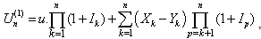 | (1.2) |
On the other hand, if the premiums are collected at the end of each period, then the surplus process  with initial surplus
  can be written as
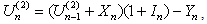 | (1.3) |
which is equivalent to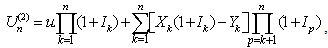 | (1.4) |
where throughout this paper, we denote  and
and  if
if  .We assume that:Assumption 1.1.
  Assumption 1.2.
  is a sequence of independent and identically distributed non – negative continuous random variables with the same distributive function
  .Assumption 1.3.
  is a homogeneous Markov chain,
  take values in a finite set of non - negative numbers
  with
with  and
and  where
where  Assumption 1.4.
  is homogeneous Markov chain,
  take values in a finite set of non - negative numbers
  with
with  and
and  where
where  Assumption 1.5.
  and
and  are assumed to be independent.We define the finite time and ultimate ruin probabilities of model (1.1) with assumption 1.1 to assumption 1.5, respectively, by
 | (1.5) |
 | (1.6) |
Similarly, we define the finite time and ultimate ruin probabilities of model (1.3) with assumption 1.1 to assumption 1.5, respectively, by | (1.7) |
 | (1.8) |
In this paper, we derive probability inequalities for  and
and  . The paper is organized as follows; in Section 2, we give recursive and integral equations for
  and
and  . In Section 3 we derive probability inequalities for
  and
and  by an inductive approach. A numerical example is given to illustrate these results in Section 4. Finally, we conclude our paper in Section 5.
2. Integral Equation for Ruin Probabilities
We first give recursive equations for  and an integral equation for
  .Theorem 2.1. If model (1.1) satisfies the assumptions 1.1 to 1.5 then for n = 1, 2, …
  | (2.1) |
and | (2.2) |
Proof.Give  Let
Let 
 ,
, .From (1.1), we have
  and
and | (2.3) |
In addition,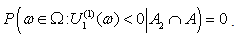 | (2.4) |
Let  be independent copies of
  ,
,  ,
,  respectively with
  Thus, (2.4) and (1.2) imply that
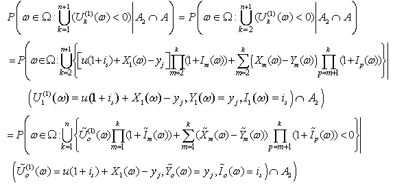 | (2.5) |
On the other hand, (1.5) implies Thus, we have
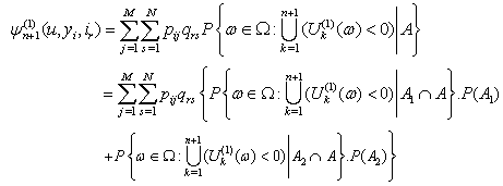 | (2.6) |
From (2.3), we have .From (2.5), we have
 Therefore, (2.6) is written as
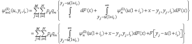 | (2.7) |
Thus, the integaral equation for  in Theorem 2.1 follows immediately from the dominated convergence theorem by letting
  in (2.7).This completes the proof Similarly, the following recursive equation for
  and integral equation for
  are hold.Theorem 2.2. If model (1.3) satisfies assumptions 1.1 to 1.5 then, for n = 1, 2, …
 | (2.8) |
and | (2.9) |
Next, we establish probability inequalities for ruin probabilities of model (1.1) and model (1.3).
3. Probability Inequalities for Ruin Probabilities
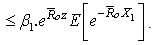
To establish probability inequalities for ruin probabilities of model (1.1), we first proof the following Lemma.Lemma 3.1. Let model (1.1) satisfy assumptions 1.1 to 1.5 and  . If, any
 ,
, and
and | (3.1) |
then there exists a unique positive constant  satisfying:
 | (3.2) |
Proof.Define  We have
 From
From  is discrete random variables and it takes values in
  then
then  has
has  -th derivative function on
  (any
(any  ).In addition,
  with
with  satisfying :
 and
and  .This implies that
  has
has  -th derivative function on
  with
with  . Thus,
  has
has  -th derivative function on
  with
with  and
and
 .This implies that
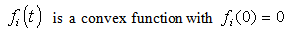 | (3.3) |
and | (3.4) |
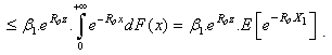
By  , we can find some constant
  such that
 Then, we can get that
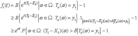 Imply
Imply | (3.5) |
From (3.3), (3.4) and (3.5) there exists a unique positive constant  satisfying (3.2).This completes the proof .Let:
  Using Lemma 3.1 and Theorem 2.1, we obtain a probability inequality for
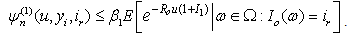
  by an inductive approach.Theorem 3.1. If model (1.1) satisfies assumptions 1.1 to 1.5,
  and (3.1) thenfor any
  ,
, and
and 
 | (3.6) |
where Proof.Firstly, we have
 .For any
  , we have
 | (3.7) |
 | (3.8) |
Then, for any  ,
, and
and  , we can write
  | (3.9) |
Thus, combining (3.8) and (3.9), we have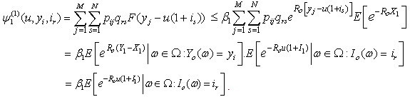 | (3.10) |
Applying an inductive hypothesis, we assume for any  ,
, and
and  ,
, | (3.11) |
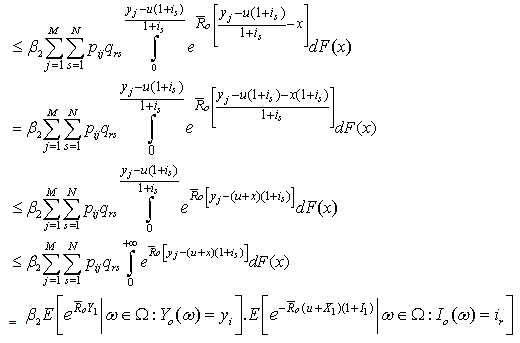
Then (3.10) implies that (3.11) holds with n = 1. For  ,
,  and
and  , we have
 where
where  ,
, and
and  For any

 then
then
 .That
.That  then
then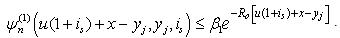 | (3.12) |
Therefore, by Lemma 3.1, (2.1), (3.7) and (3.12), we get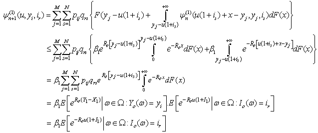 Thus
Thus Consequently, for any
  (3.11) holds. Therefore, (3.6) follows by letting
  in (3.11).This completes the proof Remark 3.1. Let
  . From
 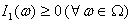 and
and  , we have
 Therefore, upper bound for ruin probability in (3.6) is better than
  .Similar to Lemma 3.1, we have Lemma 3.2.Lemma 3.2. Assume that model (1.3) satisfies assumptions 1.1 to 1.5 and
  . If any
  and
and  ,
,  and
and 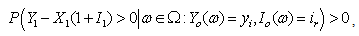 | (3.13) |
then there exists a unique positive constant  satisfying:
 Let
Let  Next, we use Lemma 3.2 and Theorem 2.2 to give a probability inequality for
  by an inductive approach.Theorem 3.2. If model (1.3) satisfies assumptions 1.1 to 1.5,
  and (3.13) then, for any
  and
and 
 | (3.14) |
where Proof.Similarly with Theorem 3.1, we have
  and any
 | (3.15) |
 | (3.16) |
Then, for any  ,
,  and
and 
 Hence
Hence | (3.17) |
Under an inductive hypothesis, we assume that  | (3.18) |
Then, (3.17) implies that (3.18) holds with n = 1. For  ,
,  and
and  , we have
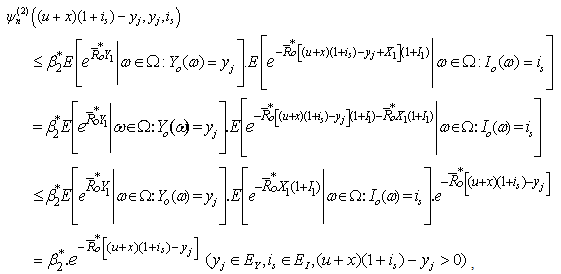 where
where  ,
, and
and  For any
 then
then 

 We get
  then
then | (3.19) |
Therefore, by Lemma 3.2, (2.8), (3.15) and (3.19), we get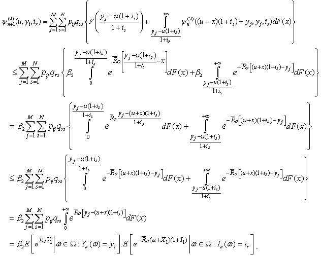 Thus
Thus Consequently, for any n =1, 2, … (3.18) holds. Therefore, (3.14) follows by letting
  in (3.18). Remark 3.2.Let
 From
From  and
and  , we have
 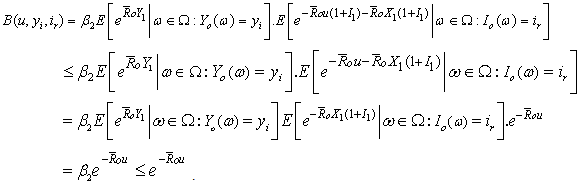 Hence, upper bound for ruin probability in (3.14) is better than
  .
.
4. A Numerical Illustration
In this section we give a numerical example to illustrate the bounds of  derived in Section 3. Let
  be a sequence of independent and identically distributed non-negative continuous random variables with the same distributive function
  .Let
.Let  be a homogeneous Markov chain such that for any
  ,
,  take values in
  with
with  having a distribution:
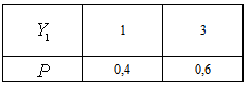 and matrix
  is given by
 Let
Let  be a homogeneous Markov chain such that for any
  ,
,  take value in
  with
with  having a distribution:
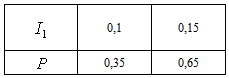 and matrix
  is given by
 Then, we have
  Therefore
 | (4.1) |
In the other hand, | (4.2) |
and  | (4.3) |
Combining (4.1), (4.2) and (4.3) imply that Lemma 3.1 holds.Next, we solve equation (3.2). Firstly, we have where
where (
( )and
)and
 Respective equation (3.2) for
  , by
, by | (4.4) |
 | (4.5) |
Using Maple, we find respective root of (3.2) for  , by
, by Hence,
  .We can apply the result of Theorem 3.1 for
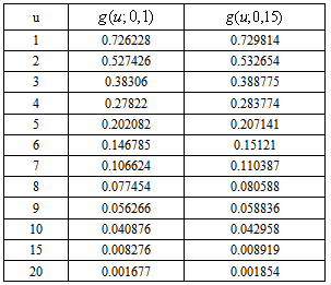
 | (4.6) |
where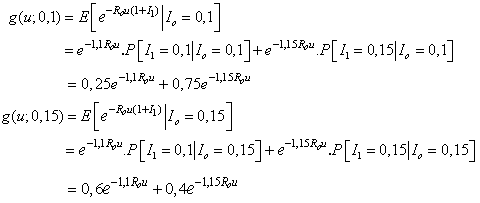 Table 1 shows values upper bounds
  of
of  for a range of value of u
5. Conclusions
Our main results in this paper are Theorem 2.1 and Theorem 2.2 giving recursive equations for  and
and  and integral equations for
  and
and  ; Theorem 3.1 and Theorem 3.2 giving probability inequalities for
  and
and  by an inductive approach. In addition, a numerical example is given illustrating Theorem 3.1.
ACKNOWLEDGMENTS
The author is thankful to the referee for providing valuable suggestions to improve the quality of the paper.In addition, the author would like to express his sincere gratitude to Professor Bui Khoi Dam for many scientific suggestions during the preparation of this paper.
References
| [1] | Albrecher, H. (1998) Dependent risks and ruin probabilities in insurance. IIASA Interim Report, IR-98-072 . |
| [2] | Asmussen, S. (2000) Ruin probabilities, World Scientific, Singapore. |
| [3] | Cai, J. (2002) Discrete time risk models under rates of interest. Probability in the Engineering and Informational Sciences, 16, 309-324. |
| [4] | Cai, J. (2002) Ruin probabilities wwith dependent rates of interest, Journal of Applied Probability, 39, 312-323. |
| [5] | Cai, J. and Dickson, D. CM (2004) Ruin Probabilities with a Markov chain interest model. Insurance: Mathematics and Economics, 35, 513-525. |
| [6] | Nyrhinen, H. (1998) Rough descriptions of ruin for a general class of surplus processes. Adv. Appl. Prob., 30 , 1008-1026. |
| [7] | Promislow, S. D. (1991) The probability of ruin in a process with dependent increments. Insurance: Mathematics and Economics, 10, 99-107. |
| [8] | Rolski, T., Schmidli, H., Schmidt, V. and Teugels, J. L.(1999) Stochastic Processes for Insuarance and Finance. John Wiley, Chichester. |
| [9] | Shaked, M. and Shanthikumar, J. (1994), Stochastic Orders and their Applications. Academic Press, San Diego. |
| [10] | Sundt, B. and Teugels, J. L (1995) Ruin estimates under interest force, Insurance: Mathematics and Economics, 16, 7-22. |
| [11] | Sundt, B. and Teugels, J. L. (1997) The adjustment function in ruin estimates under interest force. Insurance: Mathematics and Economics, 19, 85-94. |
| [12] | Xu, L. and Wang, R. (2006) Upper bounds for ruin probabilities in an autoregressive risk model with Markov chain interest rate, Journal of Industrial and Management optimization, Vol.2 No.2,165- 175. |
| [13] | Yang, H. (1999) Non – exponetial bounds for ruin probability with interest effect included, Scandinavian Actuarial Journal, 2, 66-79. |
| [14] | Willmost, G. E, Cai, J. and Lin, X.S. (2001) Lundberg Approximations for Compound Distribution with Insurance Applications. Springer – Verlag, New York. |
 Abstract
 Reference
 Full-Text PDF
 Full-text HTML
 of
of