Yucheng Liu
Department of Mechanical Engineering, University of Louisiana, Lafayette, LA 70504, USA
Correspondence to: Yucheng Liu, Department of Mechanical Engineering, University of Louisiana, Lafayette, LA 70504, USA.
| Email: |  |
Copyright © 2012 Scientific & Academic Publishing. All Rights Reserved.
Abstract
A numerical method is presented in this paper to solve linear Volterra integral equations of the second kind. In this proposed method, orthogonal Legendre polynomials are employed to approximate a solution for an unknown function in the Volterra integral equation and convert the equation to system of linear algebraic equations. The accuracy and efficiency of this method are illustrated through some numerical examples.
Keywords:
Volterra Integral Equation, Legendre Polynomial, Operational Matrix, Function Approximation
Cite this paper: Yucheng Liu, Application of Legendre Polynomials in Solving Volterra Integral Equations of the Second Kind, Applied Mathematics, Vol. 3 No. 5, 2013, pp. 157-159. doi: 10.5923/j.am.20130305.01.
1. Introduction
Linear Volterra integral equations of the second kind have the form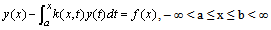 | (1) |
In solving the integral equations with given kernel k(x, t) and the function f(x), the problem is typically to find the unknown function y(x). Several numerical methods for solving these integral equations have been presented. Babolian and Shamloo[1] used operational matrices of piecewise constant orthogonal functions to solve these equations. In their method, the integral equations were transformed to Laplace form and the numerical solutions were obtained through an inversion of Laplace transform by operational matrices. Ordokhani and Razzaghi[2] developed rationalized Harr functions and used them to approximate the unknown function y(x) of the nonlinear Volterra integral equations and reduced these integral equations to a set of algebraic equations then solved them. Mestrovic and Ocvirk[3] applied the Romberg extrapolation on the quadrature method solution of linear Volterra integral equations of the second kind. Rashidinia and Zarebnia[4] proposed a method of using Sinc basis functions to solve the linear Volterra integral equation of the second kind. The numerical results showed a good convergence and verified the efficiency and accuracy of that method. Orthogonal polynomials have been widely used for function approximation. Therefore, in the solution of the Volterra integral equation, such polynomials can be applied to approximate y(t) and then convert the integral equation into a system of algebraic equations and solve it. Maleknejad et. al.[5] used Chebyshev polynomials to solve both linear and nonlinear Volterra integral equations of the second kind and illustrated the accuracy and efficiency of their method. In this paper, another general orthogonal polynomial, Legendre polynomial, is used in the solution of the linear Volterra integral equations.
2. Legendre Polynomial
Legendre polynomial is an important orthogonal polynomial with interval of orthogonality between -1 and 1, and also is considered as the eigenfunctions of singular Sturm-Liouville[6]. Matehmatically, Legendre polynomials are solutions to Legendre’s differential equation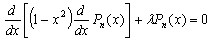 | (2) |
where the eigenvalue λ equals n(n+1). The recurrence relation of Legendre polynomials is | (3) |
and Rodrigues’ formula is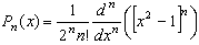 | (4) |
Because of its orthogonal properties, Legendre polynomials have been used for solving other integral equations such as Fredholm integral equations[7]. This paper employs Legendre polynomials to expand the unknown function y(x) in Eqn. (1) as Legendre polynomials series with unknown coefficients. The unknown coefficients are then determined based on the properties of the Legendre polynomials and some operational matrices. The detailed approach is demonstrated in following sections and validated through several numerical results.
3. Function Approximation
A function f(x) defined on[-1, 1] can be expanded by Legendre polynomials series as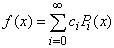 | (5) |
If the infinite series in Eqn. (5) is truncated, then we have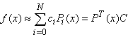 | (6) |
where C and P(x) are (N + 1) × 1 vectors given by | (7) |
In Eqn. (7) the coefficients ci are determined by Scanlon[8]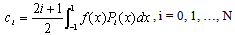 | (8) |
The kernel k(x, t) is estimated as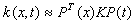 | (9) |
where K is a (N+1)×(N+1) matrix, with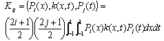 | (10) |
where (.,.) denotes the inner product.
4. Solving Volterra Integral Equations
In this section, the Volterra integral equation of the second kind (Eqn. (1)) is solved by using Legendre polynomials Pi(x). As demonstrated in above sections, the unknown function y(x), and the kernel k(x, t) are firstly approximated as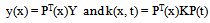 | (11) |
The integral  is approximated as
 | (12) |
Here we have to simplify .From previous researches[9, 10], we assume a (N+1) × (N+1) square matrix Z(x) whose elements zij are, which can be easily calculated based on a given x.
  | (13) |
Substituting Eqn. (11 – 13) into Eqn. (1) and have | (14) |
To find the unknown coefficient vector Y, select N + 1 collocation points xi in the interval[-1, 1] that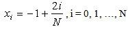 | (15) |
Eqn. (14) is therefore reduced to a system of N + 1 linear algebraic equations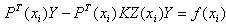 | (16) |
where PT(xi) and f(xi) are N + 1 vectors, K and Z(xi) are (N+1) × (N+1) square matrices, which can be calculated from above equations based on specified xi. The vector Y can be easily solved as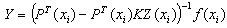 | (17) |
The unknown function y(x) is then approximated using the Legendre polynomials with coefficients Y.
5. Numerical Examples
In this section, several numerical examples of the Volterra integral equation (Eqn. (1)) are solved to illustrate the accuracy of presented method. These problems have been previously solved by Mestrovic and Maleknejad[3, 5]. All calculations are performed using Maple 11 and Matlab 7.0; the detailed steps are:1. Approximate y(x) and k(x, t) with Legendre polynomials and start with Eqn. (14) (Eqn. (11, 14)). 2. Determine the order N and select collocation points (Eqn. (15)). 3. Calculate square matrix K for given kernel k(x, t) (Eqn. (10).4. Evaluate vectors PT(xi) and f(xi), and compute square matrix Z(xi) for every collocation points xi (Eqn. (16)).5. Return to Eqn. (17) and solve Y as well as y(x).Numerical results are compared with the exact solutions and plotted in following figures to validate the proposed method.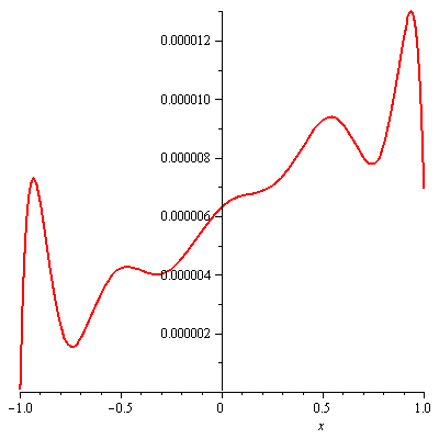 | Figure 1. Absolute error in example 1 for N = 10 |
Example 1Solve the linear Volterra integral equation of the second kind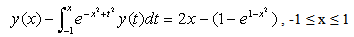 where
where 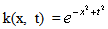 and
and 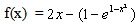 with exact solution y(x) = 2x.We solve this problem following above steps with N = 10. The obtained results are compared to the exact solution and the absolute errors between the estimated solution and the exact one are plotted in figure 1. From that figure it can be found that the errors are below 1.3 × 10⁻⁵.Example 2Solve the linear Volterra integral equation of the second kind
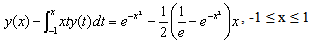 where k(x, t) = xt and
 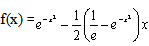 with exact solution is
  .Similarly, this problem is solved by using the proposed method and the absolute errors between the approximated solution and the exact one are displayed in figure 2. From that figure it can also be seen that the errors are below 3.0 × 10⁻⁵. Please note that in this example, for k(x, t) = xt, K is calculated as a zero square matrix. Therefore, Y is directly solved from Y = (PT(xi))-1f(xi).
  | Figure 2. Absolute error in example 2 for N = 10 |
6. Conclusions
In this paper, the linear Volterra integral equation of the second kind is solved by employing Legendre polynomials and collocation method. In the presented method, the unknown function y(x) is approximated using Legendre polynomials and the integral equation is converted to a system of algebraic equations. Detailed steps are illustrated within text step by step. As verified through numerical examples, the proposed method provides good efficiency that in order to acquire enough accuracy, we only need to convert the integral equation to the system of linear equations by order less than ten. This method can be extended and applied to solving general integral equations and equation systems with appropriate modifications.
References
| [1] | E. Babolian and A.S. Shamloo, “Numerical solution of Volterra integral and integro-differential equations of convolution type by using operational matrices of piecewise constant orthogonal functions”, Journal of Computational and Applied Mathematics, 214(2) (2008) 495 – 508. |
| [2] | Y. Ordokhani and M. Razzaghi, “Solution of nonlinear Volterra-Fredholm-Hammerstain integreal eqations via a collocation method and rationalized Haar functions”, Applied Mathematics Letters, 21(1) (2008) 4 – 9. |
| [3] | M. Mestrovic and E. Ocvirk, “An application of Romberg extrapolation on quadrature method for solving linear Volterra integral equations of the second kind”, Applied Mathematics and Computation, 194(2) (2007) 389 – 393. |
| [4] | J. Rashidinia and M. Zarebnia, “Solution of a Volterra integral equation by the Sinc-collocation method”, Journal of Computational and Applied Mathematics, 206(2) (2007) 801 – 813. |
| [5] | K. Maleknejad, S. Sohrabi, and Y. Rostami, “Numerical solution of nonlinear Volterra integral equations of the second kind by using Chebyshev polynomials”, Applied Mathematics and Computation, 188 (2007) 123 – 128. |
| [6] | R.E. Attar, “Special Functions and Orthogonal Polynomials”, Lulu Press, Morrisville, NC, 2006. |
| [7] | K. Maleknejad, K. Nouri, and M. Yousefi, “Discussion on convergence of Legendre polynomial for numerical solution of integral equations”, Applied Mathematics and Computation, 193 (2007) 335 – 339. |
| [8] | P.J. Scanlon, “An alternative form for the Legendre polynomial expansion coefficients”, Journal of Computational Physics, 1987, 69(2), 482-486. |
| [9] | A. Akyuz-Dascioglu and H.C. Yaslan, “An approximation method for the solution of nonlinear integral equations”, Applied Mathematics and Computation, 174 (2006) 619 – 629. |
| [10] | M. Sezer and S. Dogan, “Chebyshev series solution of Fredholm integral equations”, International Journal of Mathematical Education in Science and Technology, 27(5) (1996) 649 – 657. |
 Abstract
 Reference
 Full-Text PDF
 Full-text HTML