-
Paper Information
- Next Paper
- Paper Submission
-
Journal Information
- About This Journal
- Editorial Board
- Current Issue
- Archive
- Author Guidelines
- Contact Us
Applied Mathematics
p-ISSN: 2163-1409 e-ISSN: 2163-1425
2013; 3(4): 117-124
doi:10.5923/j.am.20130304.01
A Prey-predator Model with Saturating Effect of Prey on the Predator in a Restricted Habitat
 Abstract
 Reference
 Full-Text PDF
 Full-text HTML
Joy Ray1, Rifat Mahjabin1, S. M. Ashrafur Rahman1, 2
1Mathematics Discipline, University of Khulna, Khulna-9208, Bangladesh
2Department of Applied Mathematics, University of Western Ontario London ON, N6A 5B7, Canada
Correspondence to: S. M. Ashrafur Rahman, Mathematics Discipline, University of Khulna, Khulna-9208, Bangladesh.
| Email: |  |
Copyright © 2012 Scientific & Academic Publishing. All Rights Reserved.
In this paper, a prey-predator model is developed by introducing a saturating effect of prey population on predator. It is observed that saturation has great impact on the qualitative behavior of the dynamics of the population. We investigate the stability of the equilibria of the model. The global stability analysis is carried out by choosing a suitable Lyapunov function. It is found that the interior equilibrium, both prey and predator are positive, is globally asymptotically stable whenever it exists.
Keywords: Restricted Habitat, Saturating Effect, Stability, Lyapunov Function
Cite this paper: Joy Ray, Rifat Mahjabin, S. M. Ashrafur Rahman, A Prey-predator Model with Saturating Effect of Prey on the Predator in a Restricted Habitat, Applied Mathematics, Vol. 3 No. 4, 2013, pp. 117-124. doi: 10.5923/j.am.20130304.01.
Article Outline
1. Introduction
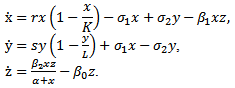
- Mathematical modelling is an area of applied mathematics that focuses on studying mathematics of the real world. The increasing study of realistic mathematical models in ecology[5, 20] is a reflection of their use in helping to understand the dynamic processes involved in such areas as predator-prey and competition interactions, renewable resource management, evolution of pesticide resistant strains, control of pests, multi-species societies, plant-herbivore systems and so on.Competition is a central role of the ecosystem where every species compete for its establishment against all species who share the same habitat and resources. Natural disaster and human induced effects are constant pressure on dynamics of the ecosystem[19, 21]. Under this pressure many species disappeared from the world and many are in great danger. Conservation of forest helps protect wild life and keep the balance in the ecosystem. In principle, part of the system of a large ecosystem would be declared reserved and rest of the system remained unreserved. To ensure the safety of any species the predators of that species are not allowed in the reserved area, where as prey can move freely between the two zones. Several researches found the effectiveness of this eco-model on the conservation of threatened wild life[8-14].How the dynamics of the wild life evolves in a controlled ecosystem gains much interest among the ecologists. Mathematical models have been playing a major role in investigating long term behaviour of the dynamics of the ecosystem[1-5]. Tyson et al. investigate the role of a specialist predator on the low densities of a prey in the cycle of prey-predator system in the boreal field[22]. Dubey et al. highlight the importance of conservation of resources by showing that fish populations can be maintained at an appropriate equilibrium level, in a habitat divided into reserved and unreserved zones, even if fishery is exploited continuously in the unreserved zone[7]. In a similar study Zhang et al. also obtained the same consequences with optimal fishing strategy[15]. Some studies focused on the protection of prey population by implementing control measures on predators[16-18]. In another study, Dubey et al. found that the reserve zone has a stabilizing effect on predator-prey interactions[6].Realizing the importance of conservation of ecosystems we further investigate the model of[6] with more realistic interactions. For convenience of study we present here the original model (1.1). Consider a prey-predator system in a habitat that divided into two zones, an unreserved zone where prey and predator can move freely, and a reserved zone where prey can live but predators are not allowed to enter the area. It is also considered that the predator is totally dependent on the prey. The dynamics of the system is governed by the following system
 | (1.1) |
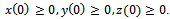 Here x and y are preys in reserved and unreserved zones respectively; z is a predator. The interaction,
  , between prey and predator is bilinear. This is also known as mass action law. In this interaction, consumption of predator increases with the number of prey. However, in reality every predator has a maximum consumption capacity. Beyond this maximum limit predator do not consume prey any more. Which can be reflected by saturating functional response defined by
  , where
  is a positive constant. The factor
  can be explained as the attack prevention ability of prey. As the number of prey x tends to infinity, this functional response becomes constant indicating the fixed amount of consumption of predator. In this paper, we modify the model (1.1) by including saturating response of prey population and investigate the effect of saturation on the dynamics of the prey-predator system. The rest of the paper is organized as follows. In Section 2, we formulate the model, which is a straight forward modification of the model (1.1). Section 3 presents the criterion of the existence of equilibria. Stability of the equilibria is analyzed in Section 4. In Section 5, the numerical simulation of the model is presented. Finally, Section 6 provides a discussion and some concluding remarks.
2. The Model with Saturating Effect
- As discussed in previous section, let
 be the density of prey species in unreserved zone,
  be the density of prey species in reserved zone and
  be the density of the predator species at any time
  . Let
. Let  be the migration rate of the prey species from unreserved to reserved zone and
  be the migration rate of the prey species from reserved to unreserved zone. It is assumed that the prey species in both zones are growing logistically. The interaction between prey and predator is assumed to be followed by the law of saturation. Then dynamics of the system is governed by the following system of ordinary differential equations:
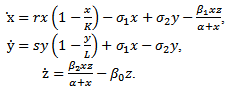 | (2.1) |
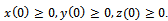 In the model (2.1), r and s are intrinsic growth rate coefficients of prey species in unreserved and reserved zones respectively; K and L are their carrying capacities.
  is depletion rate coefficient of the prey species due to the predator,
  is the natural death rate coefficient of the predator species and
  is the attack prevention ability of prey. All the parameters r, s,
  and
and  are assumed to be positive constants. With these assumptions, it can be shown that the solutions of (2.1) are positively invariant and bounded in the positive cone as stated in the following theorem. Theorem 2.1 The set
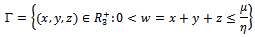 is a region of the attraction for all solution of the model (2), where
  is a constant such that
3. Existence of Equilibria
- The system (2.1) has only three nonnegative equilibria, namely
 and
and  . The trivial equilibrium
  exists obviously regardless of the parameters. Regarding the equilibrium
  , we have following existence criteria
 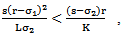 | (3.1) |
 | (3.2) |
 ) and
) and  , then,
  . Similarly, if there is no migration of the prey species from unreserved to reserved zone (i.e.
  ) and
) and  then
then  . Hence it is natural to assume that
 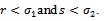 | (3.3) |
 is given by
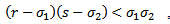
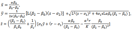 It is noted that
  to be positive, we must have
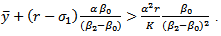 | (3.4) |
4. Stability Analysis
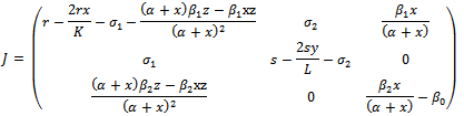
- In this section, we study the stability of equilibria. To analyze the stability of the equilibrium, we linearize the system (2.1). The Jacobian of the system (2.1) is given by,
4.1. Local Stability of 
- At
 (0, 0, 0), the Jacobian of system (2.1) becomes
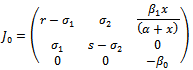 One of the eigenvalues of
  is
is  , which is negative. The sign of the other two eigenvalues or stability of
  can be determined from the trace and determinant of the sub matrix of
  given by
 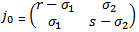 The trace of
  is negative and the determinant of
  is positive if
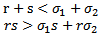 | (4.1) |
 is stable if the conditions (4.1) hold. Otherwise,
  is a unstable saddle point.
4.2. Local Stability of 
- At
 the Jacobian is given by
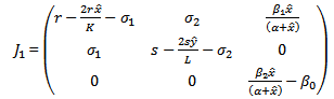 One of the eigenvalue of
  is
is  , which is negative if
 | (4.2) |
 can be determined from the trace and determinant of the sub matrix
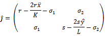 By the similar argument, the two eigenvalues of
  are negative if
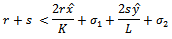 and
and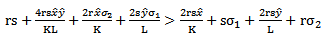 | (4.3) |
 is locally asymptotically stable, if the conditions (4.2) and (4.3) are hold. Otherwise,
  is unstable.
4.3. Global Stability of 
- We present the global stability criterion of the coexistence equilibrium. In the following theorem, we show that
 is globally asymptotically stable.Theorem 4.1 The interior equilibrium
  is globally asymptotically stable whenever it exists.Proof: Suppose that the coexistence equilibrium
  exists. We use the following positive definite function about
  for global stability.
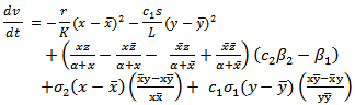
 Differentiating
  along the solutions of model (2.1), we get
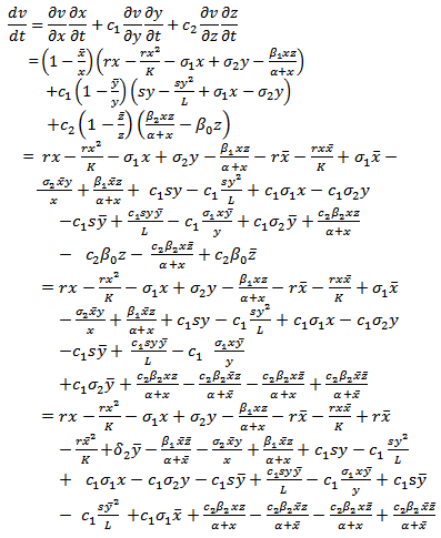 That is
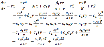 | (4.4) |
 , we have
 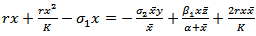 | (4.5) |
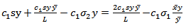 | (4.6) |
 | (4.7) |
 and
and  can further be written as,
 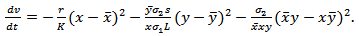 | (4.8) |
- This shows that
 , with equality holding only at the equilibrium
  . Hence v is a Lyapunov function[20] and
  is globally asymptotically stable.
5. Numerical Simulation
- In this section, we present some numerical simulations of the model (2.1) to illustrate the results obtained in the previous sections. To carry out the numerical simulation we need the parameter’s values. Since the data are not available we choose the following values of the parameters from[6] to simulate the models (1.1) and (2.1).
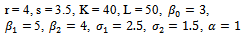 | (5.1) |
 exists with
 , and
, and . The interior equilibrium
  also exists with
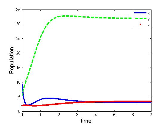
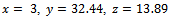 . Initially, if the predator (z) is zero, it remains zero forever. This is shown in Fig 1. However, with the positive initial values of
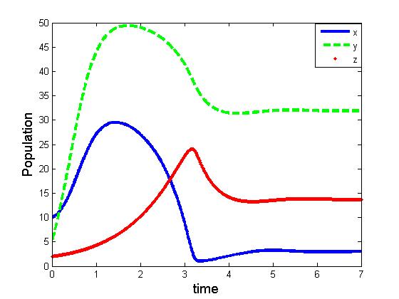
  and
and , the solutions of (2.1) approach to the equilibrium
 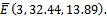 This shows that the equilibrium
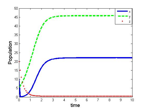
  is stable, shown in Fig 2. By changing the parameter,
  from 3.0 to 3.20 , It can be shown that the predator free equilibrium
  is stable, Fig 3. In this case, the interior equilibrium
  does not exist which is consistent with Theorem 4.1, that upon existence the equilibrium
  is globally asymptotically stable.
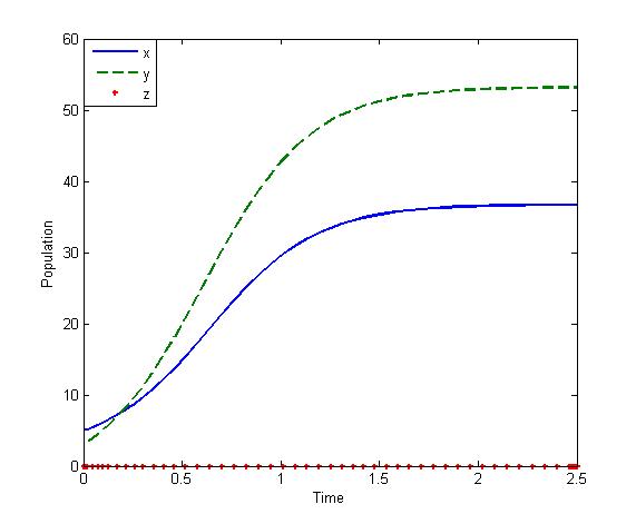 | Figure 1. Solutions of the model (2.1). Predator free state.Parameters: r =4, s=3.5, K=40, L=50, σ1=2.5, σ2=1.5, β0=3.0, β1=5.0, β2=4.0, x(0)=5, y(0)=3, z(0)=0, and α=1 |
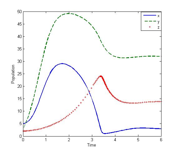 | Figure 2. Solutions of the model (2.1):State of co-existence Parameters: r =4, s=3.5, K=40, L=50, σ1=2.5, σ2=1.5, β0=3.0, β1=5.0, β2=4.0, x(0)=5, y(0)=4, z(0)=3, and α=1 |
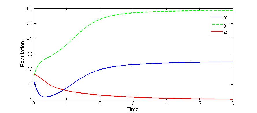 | Figure 3. Solutions of the model (2.1): Predator is disappeared. Parameters: r =4, s=3.5, K=40, L=50, σ1=3, σ2=1.5, β0=3.0, β1=5.0, β2=3.2, x(0)=10, y(0)=5, z(0)=20, and α=1 |
 | Figure 4. Solutions of the model (1.1). Parameters: r =4, s=3.5, K=40, L=50, σ1=2.5, σ2=1.5, β0=3.0, β1=4.0, β2=3.0, x(0)=5, y(0)=3, z(0)=0 |
 | Figure 5. Solutions of the model (2.1). Parameters: r =4, s=3.5, K=40, L=50, σ1=2.5, σ2=1.5, β0=2.5, β1=4.0, β2=3.0, x(0)=5, y(0)=3, z(0)=0, and α=1 |
 | Figure 6. Solutions of the model (1.1). Parameters: r =4, s=3.5, K=40, L=50, σ1=2.5, σ2=1.5, β0=3.1, β1=5.0, β2=5.50, x(0)=5, y(0)=3, z(0)=0 |
 | Figure 7. Solutions of the model (2.1):Predator free state. Parameters: r =4, s=3.5, K=40, L=50, σ1=2.5, σ2=1.5, β0=3.1, β1=5.0, β2=5.5, x(0)=5, y(0)=3, z(0)=0, and α=10. |
6. Discussion
- We developed a model to investigate the saturation effect of prey population in the dynamics of a prey-predator system. Local stability criterion of the equilibria are established through standard method. We also determined the global stability of the coexistence equilibrium. To observe the effect of saturation effect on the dynamics of the model, let us investigate some aspects of two models. In comparison, the models (1.1) and (2.1) preserve the number of equilibrium states. The equilibrium points namely
 and
and  of the corresponding models are component wise equal for both the models. However the interior equilibria
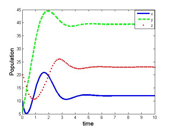
  of the two models and their stability conditions are quite different. We may also observe some significant effect of saturation from numerical exploration. Using the same set of parameter values in equation (1.1) and (2.1) it is observed in Fig 4-5 that the solutions of model (2.1) takes longer time to reach the equilibrium state than that of model (1.1). It is also noticed that the population of model (2.1) experience a large oscillation followed by small oscillations before settle down to the equilibrium state. By contrast, such effect is not observed in the solution of (1.1).Using a different parameter values in Fig 6-7, it is shown that the model (1.1) predicts co-existence of both prey and predator. By contrast, model (2.1) predicts the disappearance of predator population. This is a crucial result; because from ecological point of view we do not expect destabilization of a habitat through disappearance of a species. Thus, if a system more likely follows the model (2.1), the authority should put their attention on the predator and take some measures for the surviving of the predators.The model can be further extended to investigate the dynamics of two predators on a single prey population. We intend to report that analysis in the next project.