-
Paper Information
- Next Paper
- Paper Submission
-
Journal Information
- About This Journal
- Editorial Board
- Current Issue
- Archive
- Author Guidelines
- Contact Us
Applied Mathematics
p-ISSN: 2163-1409 e-ISSN: 2163-1425
2013; 3(3): 98-106
doi:10.5923/j.am.20130303.03
On the Estimation of Average HIV Population Using Various Bayesian Techniques
 Abstract
 Reference
 Full-Text PDF
 Full-text HTML
Gurprit Grover, Ravi Vajala, Manoj Kumar Varshney
Department of Statistics, University of Delhi, Delhi, 110007, India
Correspondence to: Ravi Vajala, Department of Statistics, University of Delhi, Delhi, 110007, India.
| Email: |  |
Copyright © 2012 Scientific & Academic Publishing. All Rights Reserved.
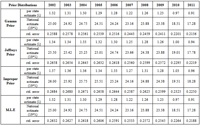
This paper models the HIV population through a Poisson distribution and obtains the expressions for the estimators of the average number of HIV individuals (Incidence Rate of HIV). Conventional methods for obtaining such estimates have used the Maximum likelihood Principle that does not take into account, any prior information about the parameter. Bayesian perspective accommodates this missing link and hence obtains the estimators where data is refined using the prior information. Three different types of prior distributions including Jeffreys non-informative priors have been considered and the corresponding estimates along with standard errors have been obtained assuming a squared error loss function. However, computational techniques like Markov Chain Monte Carlo (MCMC) have been avoided by using the Empirical Bayes Perspective. These procedures were applied on the state and year-wise data of HIV patients in India and relevant estimates are obtained and compared with actual figures. When year is considered as random variable, M.L.E proved to be better than the Bayes estimates but vice-versa is seen when states were considered as a random variable.
Keywords: Poisson Model, Human Immuno Deficiency Virus (HIV), Informative and Non-Informative Priors, Bayes Estimators, Empirical Bayes Methods
Cite this paper: Gurprit Grover, Ravi Vajala, Manoj Kumar Varshney, On the Estimation of Average HIV Population Using Various Bayesian Techniques, Applied Mathematics, Vol. 3 No. 3, 2013, pp. 98-106. doi: 10.5923/j.am.20130303.03.
Article Outline
1. Introduction
- The Kolmogrov equations for the various Birth and Death processes yield the Poisson distribution as the distribution of number of infectives at time t. This may be thought of as an intuitive result considering the fact that when we are building a model for the HIV infectives in the population, the area of opportunity is very large and the opportunity of infection is very small, so that both of them multiply to a finite quantity. This finite quantity is the average number of HIV cases in the population at time t or the HIV incidence rate per time period and may be considered as a time dependent or independent constant. The scenario may be suitably modeled through a Poisson distribution as follows:Let X denote the number of HIV infected individuals in the population. Therefore,
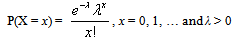 | (1) |
 or a weighted mean of observations for a sample x1, …, xn of n observations. Moreover, despite satisfying the properties of a good estimator asymptotically, the Maximum likelihood estimator (M.L.E) fails to take into account any additional information available on the parameter λ prior to taking the sample. This additional information may be incorporated into the estimation process by the so-called prior distribution and hence Bayesian approach may be used to evolve a much more refined estimator. Bayesian methods do not require large samples or asymptotics for their validity. They allow for incorporation of expert knowledge through the specification of prior distribution.Classical M.L.E approach to the problem of estimation relies on an estimator which is obtained theoretically and remains the same for whatever may be the data set. However, Bayesian approach obtains a separate set of estimators for every set of prior information and adjusts these estimators for changes in the data set. Such an estimator provides a logical alternative because it not only incorporates the additional information on the parameter, but also relies on the data to a great extent.
2. Bayes Approach for Estimating HIV Incidence Using Various Prior Distributions
- The use of prior distributions is the best way to summarize the available information (or rather lack of information) about the parameter of interest i.e., average number of HIV persons in the population. It may be helpful in incorporating the experiences from previous studies or subjective beliefs of the experimenter into the analysis. These beliefs may be put into various kinds of functional forms depending on the amount of information available.Let xi denote the number of HIV infected individuals in the population for the ith entity/time point, with probability P(xi | λ) where λ is the parameter denoting the average number of HIV infected individuals in the population. Let the prior probability (or "unconditional" or "marginal" probability) of λ be P(λ) and the joint distribution of x1, x2, …, xn be P(| λ ). Then the posterior density of λ is given by
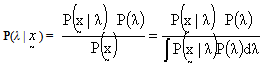 | (2) |
 does not equal zero.When substantial information about the average HIV cases is available, we may look at the (Natural) Conjugate Priors wherein the functional form of the prior and posterior remains same and when no information is available, we may consider the Non-informative Prior (Jeffreys)[10].The subsequent sections develop theory for modeling the HIV incidence λ, using various prior distributions in the population. This prior information is refined to posterior distribution by means of additional information provided by the data and estimates of λ are obtained from the posterior distribution. The estimates are obtained so as to provide minimum risk (which is expected loss) with respect to the posterior distribution. Of course, there is no consensus opinion on defining the loss, although the Quadratic loss is popularly used and found to be sufficient in majority of the situations.
2.1. Conjugate Prior for Modeling HIV Incidence
- Cole et. al[18] and Berry et al.[3] had used the Gamma distribution as a prior for the incidence of HIV infection and multiplied it with a pseudo-person-time to find the average number of recent HIV infections. The estimates were obtained using the Markov Chain Monte Carlo (MCMC) procedures. Kpozhouen et al.[2] attempted to test the Bayesian approach as a tool for optimizing management of a chemoprophylaxis trial in HIV infection by allowing interim analysis with a reduced number of patients or follow-up time. The Bayesian proportional hazards model was considered for this purpose. The unknown coefficients of the covariates and the baseline cumulative incidence were assigned three different kinds of prior distributions. Gamma prior was assumed for the baseline cumulative incidence since the variable under consideration followed Poisson distribution and also to facilitate the determination of conjugated distribution. Finally, posterior distribution and the estimates of the parameters (as well as hyperparameters) were obtained using Markov Chain Monte-Carlo (MCMC) methods. White et al.[16] developed an age-stratified model that accounts for transmission due to unsafe injections, unsafe transfusions, and mother-to child transmission. The confidence intervals for HIV incidence rates with respect to unsafe injections were based on the Poisson assumption with a Gamma prior. The estimates of relative contribution of HIV-contaminated injections, and other routes of HIV transmission in this age-structured transmission model were obtained using the MCMC techniques. Grover et al.[9] used the Bayesian approach for estimating the proportion of HIV infected population converting to AIDS. They had modeled the number of HIV infected persons using Binomial distribution and assumed the beta distribution as a conjugated prior for the proportion of HIV infected population converting to AIDS. Finally Maximum likelihood estimates were for the posterior distribution.Even though the widespread use of Computers in analysis have highlighted the importance and popularized the use of MCMC techniques, the procedure itself seems to be complex. Moreover, at times MCMC procedures involve large number of iterations and still fail to converge to any particular value. We present an easy method of obtaining the estimates of the parameters by using the Empirical Bayes approach[17] as this will save the time and complexities of an MCMC technique. The aim of suggesting the Empirical Bayes approach is not to portray the MCMC procedures in poor light, but is solely intended to provide an easy and convenient alternative. Bartolucci et al.[1] had used the Empirical Bayes analysis for estimation of incidence and intervention parameters for the Intervened Poisson (IP) model.Let us assume that the prior distribution for HIV incidence rate λ follows a Gamma distribution with parameters (α, β). On using the Bayes theorem, for a given set of data x1,… , xn, the posterior distribution of λ| x1, …, xn becomes Gamma
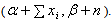 The posterior mean of the distribution is
  which provides an estimate of λ with variance
 The problem in finding the estimator of intensity λ is that it is based on the data as well as the parameters of the prior distribution α and β (known as hyperparameters). Authors[16, 18] of related studies have, on the basis of their past knowledge, judgment or intuition taken various predetermined values for these hyperparameters and obtained the estimate of the average HIV cases. These estimators were further studied for robustness with respect to the prior parameters. However, we believe that the information about the parameters of interest lies in the data itself and hence the hyperparameters have been estimated using the Empirical Bayesian Procedure[17].Let
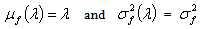
 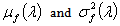 denote the conditional mean and variance of the random variable X which denotes the HIV cases in the population. Let
  denote the marginal mean and variance of these HIV cases. Assuming that these quantities exist, we have
 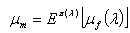 | (3) |
 | (4) |
 then,
then, 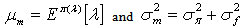 Therefore the estimates of the hyperparameters when the prior distribution of λ is Gamma(α, β) are obtained as
 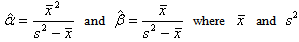 are the sample mean and variance respectively. These may in turn be used to find the estimate of HIV incidence rate along with its standard error.
2.2. Non-Informative Priors for Modelling HIV Incidence
- Kpozhouen et al.[2] used three different kind of prior distributions, one being a non-informative prior to assess the efficacy of Cotrimoxazole prophylaxis in reducing severe morbidity in adults at early stages of human immunodeficiency virus infection. The authors modeled the intensity of serious events (mortality) using the Bayesian proportional hazards model proposed by Spiegelhalter et al. (1996) and used the non-informative prior to represent the weak prior information on the coefficients of the covariates of the model. Many other authors have used the non-informative priors in terms of assigning negligible values to the parameters of the conjugate/informative prior distributions. However, none of them have modeled weak prior information in the lines of Jeffreys perspective which is a formal and admissible approach to specifying negligible information on the parameter of interest.When prior information about the HIV incidence parameter
 is not available and the intention is to use the available clinical data to determine the parameter, Harold Jeffreys[10] approach may be used to obtain the following non-subjective reference prior in terms of the Fisher’s Information matrix:
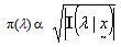 | (5) |
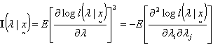 is the Fisher’s Information matrix.Therefore, the prior distribution for the HIV incidence rate (λ) according to Jeffrey’s rule may be taken as
  Using the Bayes rule, the posterior distribution is obtained as (λ|x1, …, xn ) ~ Gamma(
 ). The posterior mean of the distribution is
  which provides an estimate of λ with variance
 The situation of no prior information about the Incidence rate λ, may be also modeled through the improper prior,
  where 0 ≤ λ < ∞ for which the posterior distribution is given by (λ|x1, …, xn ) ~ Gamma
  The estimate of the HIV incidence rate is then
  with variance
  Also, in case of large sample sizes, Brenner et al.[4], Fraser and McDunnough[8] gives the asymptotic posterior distribution for the HIV incidence parameter
  on assuming non informative prior.If
  is the M.L.E of
  and prior density of
  is non-informative (or likelihood dominates the prior density), then the posterior density of
  is given by
  | x1, …, xn ~ Normal
 where L(
 ) is the logarithm of likelihood of (
 | x).Using this result, we obtain the posterior distribution of the HIV incidence as
 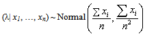 | (6) |
 with variance
  which is the Maximum Likelihood Estimator of
  .The objective of using these non-informative priors is to highlight the 'weak' or 'negligible' information over 'no' prior information as assumed while obtaining M.L.E. Also, this paper assumes an informative prior modeled by Gamma distribution in comparison with weak (Jeffreys), negligible (Improper) and no (M.L.E) prior information. The consideration for these non-informative priors is to bridge the gap between substantial amount of information as compared to no information. Various other informative priors could also have been considered for this purpose but then, these could also be obtained by giving suitable values to the parameters of Gamma distribution being one from the exponential class of distributions. In such situations, the solution would simply be obtained by doing a grid search for the best values of hyperparameters that will yield minimum standard errors of the estimators. However, doing so would dilute the concept of Empirical Bayes procedure which recommends for the estimation of hyperparameters from the sample itself.
3. Application
- The year-wise record (2002-2011) of the number of HIV patients across 19 States/Union Territories of India have been taken from the National AIDS Control Organisation (NACO)[13] and National Institute of Medical Statistics (NIMS)[11]. NACO is an agency that is committed to contain the spread of HIV in India by building an all-encompassing response reaching out to diverse populations. They strive to provide people with accurate, complete and consistent information about HIV, promote use of condoms for protection, and emphasise treatment of sexually transmitted diseases. National Institute of Medical Statistics (NIMS) aims to promote and undertake research in statistical techniques and methodology in the field of health research, exercise surveillance to ensure the statistical adequacy and validity in various programmes of the Government of India. One of their main thrust areas is modelling, estimation and projection of HIV/AIDS.
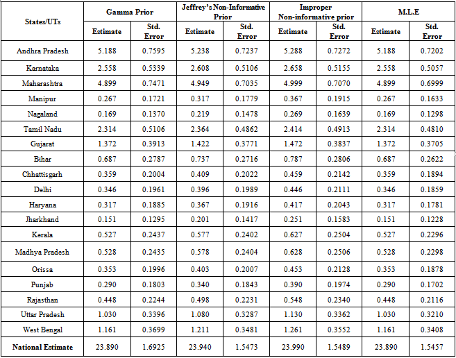
4. Results and Discussion
|
|
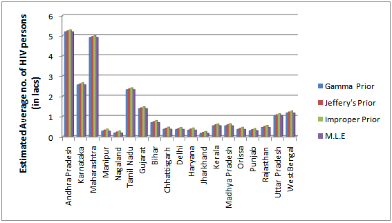 | Figure 1. Bayes estimates of the average HIV persons in various states/UT’s of India |
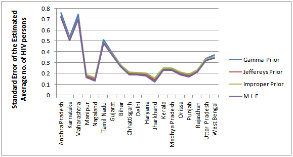 | Figure 2. Estimated Standard Error for the Bayes estimates of the average HIV persons in various states/UT’s of India |
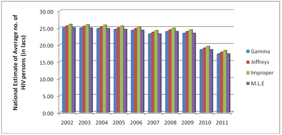 | Figure 3. Bayes estimates of the average HIV persons in India for the years 2002-2011 |
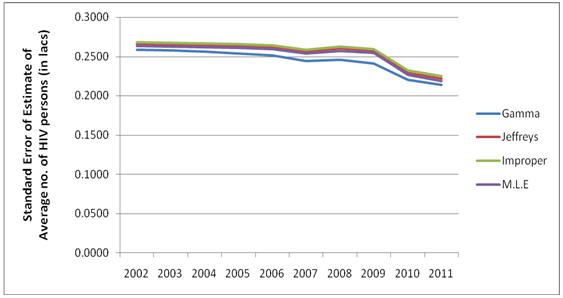 | Figure 4. Estimated Standard Error for the Bayes estimates of the average HIV persons in India for the years 2002-2011 |
|
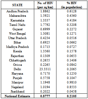
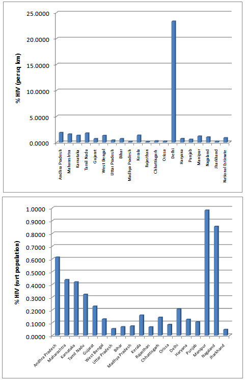 | Figure 5. Estimated % HIV with respect to Area(sq. Km) and Population |
5. Conclusions
- From the results, we note that the average number of HIV infected persons in India is declining over the years. Before coming to any conclusion on this, it may be explored whether the decrease is indeed a good sign or is a situation where they are either dying or converting to AIDS. It may also be noted that the states of Andhra Pradesh and Maharashtra have recorded high incidence of HIV cases while the lowest is seen in the Jharkhand and Nagaland. The high prevalence states of Andhra Pradesh, Maharashtra, Karnataka and Tamil Nadu show an increase in the incidence in 2011 as compared to 2009. Delhi records the highest prevalence in terms of the number of HIV cases per square Kilometer area while the lowest is seen in Rajasthan. In terms of population of each state, the highest percentage of HIV cases are seen in Manipur and Nagaland while the lowest is seen in Jharkhand.The results invariably strike a balance between Classical and Bayesian procedures by not discriminating one over the other. However, it may be noted that the Bayesian procedure is a fairly general procedure which may encompass the classical procedure by simply making assumptions on the hyperparameters. This paper obtains very good estimates of the HIV infection rate by relating it to the number of infected people and hence, subject to the assumptions of constant infection rate, prior distributions provides a good utility in the estimation procedure.Even though, this procedure can be generalized for calculating the national averages of HIV infectives, further improvements may be done by developing a procedure that incorporates time dependent Incidence Rate in the Poisson model. Such a model would refine the Bayes estimators to perform well, even for a time-series data. The incidence rate may be verified for its dependence on certain covariates and suitable Bayesian approach may be applied to it. Also, the estimators may further be improved to accommodate the case of incomplete data sets.