1. Introduction

The accelerating increase in number of car owners results in considerable growth of traffic volume, regular traffic congestion and advance in the cost of motor trucking. Cities usually develop according to the following consistent pattern: at an early stage the directions of arterial streets are laid but later the urban transportation infrastructure itself starts dictating the directional development. Therefore, optimal planning of networks and optimization of paths gain in importance. The problem of rational employment of already existing urban transportation networks by optimal organization of traffic is also urgent.

Mathematical models applied for analyzingtransportation networks vary according to the problems solved, mathematical apparatus, data used, and specification of traffic description (e.g.[1-2, 4-9, 16, 17]).The first macroscopic model was suggested by M. Lighthill and G. Whitham[8] in the middle of the last century parallel with the first microscopic models (‘follow-the-leader’ theory) which explicitly derived an equation of motion for each individual vehicle (А. Reshel, L. Pipes, D. Gazis and others).

Frank A. Haigt[5] was the first to establish the mathematical investigation of traffic flow as a separate section of applied mathematics. At present there is voluminous literature on the subject.

In order to efficiently control urban traffic flows and choose the optimal solutions of designing transportations networks we should consider a wide range of the flow features as well as the laws of impact of both external and internal factors on dynamic characteristics of traffic flow (e.g.[9],[16],[17]). The problems arise due to instability of traffic flow and divergence of the criteria of traffic control quality. The travel time for a concrete path is made up of the delays at intersections and the time of motion from one intersection to another. By reducing the waiting time at intersections we could optimize the total travel time. Therefore, developing a microscopic model of transportation dynamics in the nodes and estimation of their influence on the network flows distribution seems to be relevant.

2. A Graph Representation of Transportation Network

In stochastic models a traffic flow is defined as the result of interaction of vehicles on the segments of transportation network. A network is a graph each edge of which is assigned to a certain number. A flow is a certain function prescribed for the graph edges (e.g.[12]). In the case studied, the flow in the graph is given as a function of density of arrival distribution (arrival times of service requests).

We hold that time intervals distribution in each customer flow (channel) obeying the Erlang distribution (e.g.[11]) is:

(1)

This law allows us to describe flows of rather high density. For example, the assumption of time intervals distribution for vehicles moving in succession according to the Erlang distribution is true for the intensity of 500 vehicles per hour on each lane.

We will refer to the network flows as ‘non-conflict’ if they are not crossed in the given sector of the network, and as ‘conflict’ otherwise. We will consider the node-points – the points of sources or consumption of information and those of conflict flows crossing – to be the vertices of a graph. The node-points are formed by crossing of multichannel lines.

Let us consider a node-point (NP) in which the conflict flows are crossed as follows: a number of flows (the main ones) are freely passing the NP. The customers of the rest of flows (the secondary ones) are expecting sufficient time intervals between arrivals of main flows in order to cross the NP. We will call such a node-point a ‘type 1 node’, as in[10, 13, 15].

We will call a node-point in which traffic is alternately blocked for one of the non conflict flow group for a fixed time to enable crossing a ‘type 2 node’, as in[10, 13, 15].

Let:

= set of graph edges,

= set of nodes.

Then, a edge is part of a multichannel line between two nodes. Assign the identification numbers , to the lines. Then . And the graph could be given as the following combined matrices:

2.1.

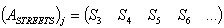
where

1) № = number of the matrix line corresponding to the number of the graph edge linking Nodes 1 and 2 (the number of lines equals the number of edges);

2) S₁ и S₂ = intersected lines forming Node 1;

3) S₃ и S₄ – intersected lines forming Node 2;

4) C = node type;

5) Pr = priority (main or secondary line);

6) L = length of edge;

7) Col = number of flows on the edge;

8) AL = admissibility of turning to the left from Direction A at Node 1;

9) AS = admissibility of direct motion from Direction A at Node 2;

10) AR = admissibility of turning to the right from Direction A at Node 2;

11)λА1, λА2, etc. = parameter λ in Direction А;

12) kA1, kA2, etc. = parameter k in Direction А;

13) BL = admissibility of turning to the left from Direction B at Node 1;

14) BS = admissibility of direct motion from Direction B at Node 1;

15) BR = admissibility of turning to the left from Direction B at Node 1;

16)λ1, λВ2 etc. = parameter λ in Direction B;

17) kB1, kB2 etc. = parameter k in Direction В.

2.2.

where

1) The line number is the number of the edge connecting the type 1 and 2 nodes in the matrix ;

2) S1 и S2 = intersected lines forming Node 1;

3) λCline1, λCline2 etc. = parameter λ of flows arriving at Node 1 in Direction C of the line crossing the given edge in Node 1;

4) kC line1, kC line2 etc. = parameter k of flows arriving at Node 1 in Direction C of the line crossing the given edge in Node 1;

5) λD line1, λD line2 etc. = parameter λ of flows arriving at Node 1 in Direction D of the line crossing the given edge in Node 1;

6) kD line1, kD line2 etc. = parameter k of flows arriving at Node 1 in Direction C of the line crossing the given edge in Node 1.

3. Optimisation of Flows Distribution in the Network

3.1. Determination of the Optimal Flow Distribution in a Node

Let us consider the following problem: we must find out the optimal distribution of flows for a given node from the known methods of the set.

Depending on the aim pursued the criteria of optimization can be:

1) = weight of the vertex (node-point) for the flow of the given direction;

2) = weight of the vertex;

3) = mean delay of request in the chosen directions.

For the type 1 node:

1) , where М = set of chosen directions;

2) , where = set of all directions;

3) , where М = set of chosen directions.

Here we used the following notation (as in[10]): = mean delay (seconds) at a node of one request of a secondary direction with λ and k parameters of distribution:

For the type 2 node:

1) , where М = set of chosen directions, ;

2) ;

3) , where М = set of chosen directions, .

Here we used the following notations (as in[10]): (requests per second) = the total delay of all requests of a given flow for one regulated cycle ;

= number of requests arriving at a given point of road for the time interval (0; t).

Let: the given vertex (node-point) (with the order precision of). The information about incoming flows is given in he matrices and.

Lemma 1. The Erlang distribution parameters for incoming flows of the vertex are given:

1) in the matrix in the line– in Direction В;

2) in the matrix in the line in Directions С and D;

3) in the matrix in the line – in Direction A.

The optimal flow distribution in the node is the solution to the problem (depending on the pursued objective):

1) ;

2) ;

3) .

3.2. Selection of the Optimal Parameters of the Type 2 Node Operation

Let us set the following task of optimization of the type 2 node operation: to minimize the total hour delay of all requests in the given node on condition of absence of congestion for each flow:

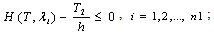(2)

(3)

where = number of flows of Line №1; = number of flows of Line №2. It is necessary also to fulfill the condition: , where М = the minimum time (seconds) necessary for a request to pass the type 2 node.

The problem of mathematical (non-linear) programming is:

(4)

(5)

The results obtained are the optimal values of operation parameters.

Specify the algorithm of numerical solution to the problem (4-5) as a relaxation process – the process of construction of successive approximations for which и.

Step 1. Specify initial values:

and

;

and the values for fulfillment of the algorithm ;;.

Step 2. Find numerically (for example, by half-division method) the solution to the equation, meeting the condition: .

Step 3. Check the fulfillment of other inequalities of the system with restrictions:

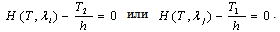
Step 4. If the conditions of Step 3 are fulfilled, compute and go to Step 5. If the conditions of Step 3 are not fulfilled, then find numerically (for example, by half-division method) the solution to the equation , meeting the condition: ; check the fulfillment of other inequalities of the system with restrictions:

Then compute and go to Step 5.

Step 5. Assume (initial value) and find numerically the solution to the equation:

The new value .

Step 6. Repeat Steps 2-4 until .

The author has proved that the successive approximations meet the conditions of convergence with the optimal solution:

.

3.3. Determination of the Critical Values of the Erlang Distribution Parameters for the Type 2 Node

As stated above, there is no congestion in the type 2 node under certain conditions (2-3). In the case where time intervals are distributed according to Erlang law (1), the given conditions are identical with the following inequality system:

(6)

Since , the approximate solution to the system for λ parameter (with k parameter being known) is:

(7)

If necessary, the value of λ parameter of the Erlang distribution for each flow preventing congestion in the type 2 node can be found numerically with any precision by solving the equation:

(8)

3.4. Selection of the Optimal Path for Flows in the Given Network (from the Preset Number)

Assume there are a limited number of certain routs , from the node to the node given by enumeration of nodes in the order of their passing by the flow requests.

Let the optimization criterion be the following function:

=weight of path, i. e. time spent on passing the given path,

where = weight of the vertex (node-point)for the flow of the given direction;;

= weight of the edge for the flow of the given direction;

= set of edges of the path;

= set of nodes of the path.

Then the optimal path is determined by the solution to the following problem:

Information about the network necessary for computation is given in two connected matrices и.

3.5. Determination of the Optimal Path between Two Nodes

Let us set the following task : to find the path from the vertex to the vertex, meeting condition: . Unlike the problem of the previous point, only the initial vertex and final vertex of the path are specified.

Take into account that the chosen graph representation allows for each node to be adjacent to four other nodes at most. A node is shown as an intersection of two lines and.

Lemma 2. Let:

, (with the order precision of,).

The nodes х and у are adjacent only when the matrix has the following row:

or

.

Lemma 3. Let:

, , (with the order precision of, ,).

In the graph there is a path, where х и у, у and z are adjacent nodes only when the following conditions are fulfilled:

Case 1)

;

The initial data are given in the following rows of the matrix:

; ;;

;

Case 2)

;

The initial data are given in the following rows of the matrix:

; ;

;;

Case 3)

;

The initial data are given in the following rows of the matrix:

; ;;

;;

Case 4)

;

The initial data are given in the following rows of the matrix:

; ;;

;;

Case 5)

;;

The initial data are given in the following rows of the matrix:

; ;;

; ;

Case 6)

; ;

The initial data are given in the following rows of the matrix:

; ;

;;

Case 7)

;;

The initial data are given in the following rows of the matrix:

; ;;

;;

Case 8)

;;

The initial data are given in the following rows of the matrix:

; ;;

;;

Case 9)

;;

The initial data are given in the following rows of the matrix:

; ;;

; ;

Case 10)

;;

The initial data are given in the following rows of the matrix:

; ;

;;

Case 11)

;;

The initial data are given in the following rows of the matrix:

; ;;

;;

Case 12)

;;

The initial data are given in the following rows of the matrix:

; ;;

;.

Each edge of the graph is assigned to the number – edge length; if the nodes are not linked by an edge then l(x,y) = ∞.

In the course of fulfillment of the algorithm, the graph vertices and edges are colored and the values d(x) are computed which equal to the shortest path from vertex s= to vertex х which only includes the colored vertices:

.

In our case: l(x, y) = mean travel time of requests of the flow from vertex x to vertex y taking into account the delay at vertex х.

The data necessary for solution to the problem will be stored in two arrays:

MPlus – data on the nodes having permanent marks;

MMinus – data on the nodes having temporal marks.

Each element of array has the following structure:

и

Str1 = line along which traffic has been flowing to the given node;

Str2 = line, intersecting Str1;

TimeCr = travel time d(x) to the given node from the initial point of the path;

Trassa – list of the nodes passed.

Step 1. Specify the start and finish of the path. The initial node is denoted as n = 0 in the array MPlus and 4n in the array MMinus.

Step 2. Define all node-points adjacent to node n^th (Lemma 1) and record their data in the array MMinus numbered as (4n + 1), (4n + 2), (4n + 3).

If vertices are not adjacent or traffic in this direction is banned then l(x,y) = ∞.

Step 3. Compute the travel time from node n^th to all adjacent nodes which are not recorded in the array MMinus.

Step 4. Select the minimum element in the field MMinus.TimeCr and record the data on a certain node in the array MPlus numbered as (n+1). Delete the data on this node from the array MMinus.

Step 5. Repeat Steps 2-4 until node (n+1) in the array MPlus coincides with the end of path. Then finish computing.

Step 6. Display the array MPlus – the list of nodes thru which the shortest path between the two given points of network goes.

The given algorithm is author's modification of Dijkstra’s algorithm[3]. It is an iterative procedure where each vertex is marked – either by a permanent mark which shows the distance from this node to a particular node or by a temporary mark when this distance is estimated from above.

The implementation of the algorithm needs n² operations (n is a number of the graph vertices).

3.6. Determination of the Optimal Scheme of Flows Distribution in the Given Network (from the Preset Number)

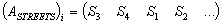
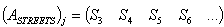
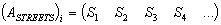
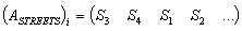
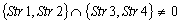
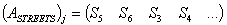
Specify the sub-graph to be reorganized. Possible variants of reorganization of flow distribution in the network are presented in the matrices и,.

If reorganization is aimed at minimizing the delays at nodes, then the criterion for optimization is he sum of nodes weights:

.

The optimal scheme of flow distribution in the network is the solution to the problem:

.

If reorganization is aimed at optimization of traffic flow along the given path in the network, then the weight of path, i.e. the time spent on passing the given path should be taken as target function:

where: = weight of vertex (node-point) for the flow in the given direction;

= weight of edge for the flow in the given direction;

= set of edges of the path;

= set of vertices of the path.

Then the optimal scheme of flow distribution in the network is the solution to the problem:

4. Conclusions

The above considered optimization problems present the probabilistic model of traffic flow developed by the author (e.g.[10, 13-15]). This model is based upon the hypothesis about the Erlang time distribution for requests arriving in succession. The adequacy of this hypothesis for traffic flows was proved by experiments. The virtue of the developed model is the minimal number of initial data necessary for computing the indices of quality of the network operation. The suggested graph representation of network allows us to solve the problems on optimization of traffic flows by optimal distribution in the nodes. If there are data files for a certain road segment in the urban transportation network organized according to the matrices и , it will be easy to implement the algorithms of solutions to these problems using computer environment, e.g. DELPHI.