-
Paper Information
- Next Paper
- Paper Submission
-
Journal Information
- About This Journal
- Editorial Board
- Current Issue
- Archive
- Author Guidelines
- Contact Us
Applied Mathematics
p-ISSN: 2163-1409 e-ISSN: 2163-1425
2013; 3(1): 1-11
doi:10.5923/j.am.20130301.01
Comparing up and Down Milling Modes of End-Milling Using Temporal Finite Element Analysis
 Abstract
 Reference
 Full-Text PDF
 Full-text HTML
Chigbogu G. Ozoegwu, Sam N. Omenyi, Sunday M. Ofochebe, Chinonso H. Achebe
Department of Mechanical Engineering, Nnamdi Azikiwe University Awka, PMB 5025 Anambra state, Nigeria
Correspondence to: Chigbogu G. Ozoegwu, Department of Mechanical Engineering, Nnamdi Azikiwe University Awka, PMB 5025 Anambra state, Nigeria.
| Email: |  |
Copyright © 2012 Scientific & Academic Publishing. All Rights Reserved.
Two types of end milling at partial radial immersion are distinguished in this work, namely; up and down end-milling. They are theoretically given comparative study for a three tooth end miller operating at 0.5, 0.75 and 0.8 radial immersions. 0.5 and 0.8 radial immersion conditions are chosen so that analysis covers situations in which repeat and continuous tool engagements occur while 0.75 radial immersion just precludes tool free flight. It results from analysis that the down end-milling mode is better favoured for workshop application than the up end-milling mode from both standpoints of cutting force and chatter stability. This superiority in chatter stability is quantified by making use of the Simpson’s rule to establish that switching from up end-milling mode to down end-milling mode at 0.5 radial immersion almost doubles the possibility of chatter free milling while at 0.75 and 0.8 radial immersions this possibility almost triples. This result conforms to the age long recognition from workshop practices that climb milling operations are much more stable than conventional milling operations. Validation of the resulting stability charts is conducted via MATLAB dde23 time domain numerical analysis of selected points on the parameter plane of spindle speed and depth of cut.
Keywords: Up end-milling, Down End-milling, Temporal Finite Elements, Phase Trajectories, Simpson’s Rule
Cite this paper: Chigbogu G. Ozoegwu, Sam N. Omenyi, Sunday M. Ofochebe, Chinonso H. Achebe, Comparing up and Down Milling Modes of End-Milling Using Temporal Finite Element Analysis, Applied Mathematics, Vol. 3 No. 1, 2013, pp. 1-11. doi: 10.5923/j.am.20130301.01.
Article Outline
1. Introduction
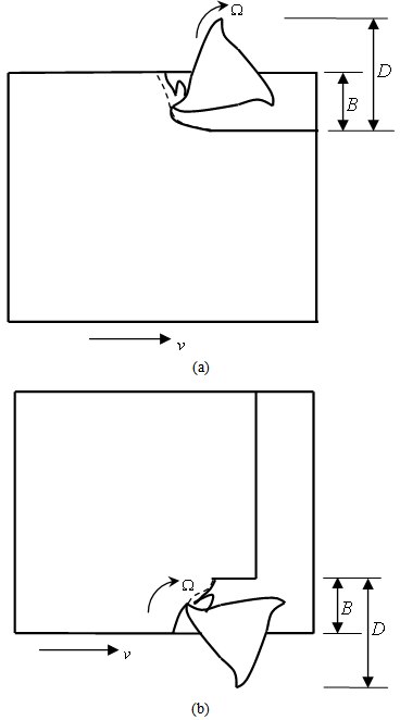
- Machining is needed for the production of specialized components in the aerospace, marine, automobile and other industries. For this reason best mode of machining is sought after for best productivity and quality of components. Among other methods of machining, end milling is extensively used in the industry. In end milling a machined surface that is at right angle with the cutter axis results as shown Figure 1. Milling cutters equipped with shanks for mounting on the spindle are utilized for end milling.Two types of end-milling at partial radial immersion are distinguished as shown in figure 2. Milling operation as depicted in figure 2.a dynamically looks like the conventional milling since workpiece feed is in opposite direction to cutter rotation at advent of tooth-workpiece engagement. Chip thickness progressively grows from zero to non-zero values as feed progresses in this type of milling. The end milling process of figure 2.b dynamically resembles the climb milling being that workpiece feed is in the same direction as cutter rotation at inception of a tooth-workpiece engagement. Chip thickness starts from non-zero value and ends at zero value in this type of milling. These milling processes will thus be referred to in this work as up end-milling and down end-milling respectively. Radial immersion
 is defined for these milling processes to mean the ratio of the radial depth of cut to the tool diameter. The aim here is to compare the cutting forces and stability of both types of end milling process for a three tooth milling tool at half, three-quarters and four-fifths radial immersions. The first major difference between this work and others is that the cutting force of the non-chattered down end-milling and up end-milling are compared. It is suggested that there is less possibility of fatigue in the down end-milling mode since its magnitude of unperturbed cutting force is always less than that of the up end-milling at all radial immersions.The superiority of conventional milling over climb milling in terms of surface quality of component in workshop practice is long known and documented[1-3]. It is noted by Joshi[2] that conventional milling has fixture or clamping problems that is entirely absent in climb milling. This is due to the lift effect cutting forces have on the workpiece in conventional milling. Miller and Miller[3] wrote that climb milling allows faster material removal rate and surface finish than conventional milling. The poorer surface finish in conventional milling is attributed to tooth-workpiece rubbing that occurs before active engagement. The fixture and rubbing-induced surface problem of conventional milling are not expected in up end-milling since the machined surface is at right angle with the cutter axis.The dynamic resemblance of up and down end-milling with conventional and climb milling respectively is considered to mean resemblance in stability. Analysis shows that domain of chatter stability of down milling mode is much greater than that of up milling mode at all the studied radial immersion conditions. The point thus made in this work is that the superiority of surface finish in climb milling over that in conventional milling is partly due to less possibility of chatter or unstable self –excited vibrations in the former. This is another contribution of this work.
 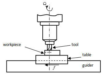 | Figure 1. End-Milling |
 | Figure 2. Two End-Milling Modes. (A) Up End-Milling; (B) Down End-Milling |
 while at 0.75 and 0.8 radial immersions this possibility almost triples in the same spindle speed range.
2. Mathematical Model of Periodic Cutting Force
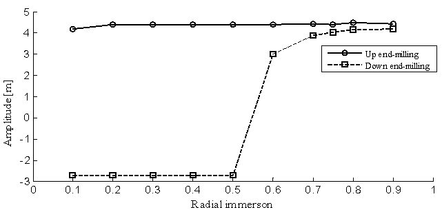
- End-milling process as depicted in figure 3 is a multi-toothed cutting operation. The tool is given a spindle speed
 in revolutions per minute while the workpiece has a prescribed feed velocity
  imparted on it via the worktable.
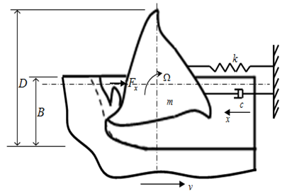 | Figure 3. Dynamical Model Of End-Milling |
 tooth of the tool where the normal and tangential components are designated
  and
and  respectively. The
  component of cutting force for the tool thus becomes
 | (1) |
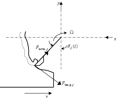 | Figure 4. Milling Tooth-Workpiece Disposition |
 is the number teeth on the milling tool indexed with the values
  . The instantaneous angular position of a tooth
  is
is  . In this work
  is measured clockwise relative to the negative
  axis to give
 | (2) |
 is the initial angular position of the tooth indexed1. Screen or switching function for the
  tooth
tooth  could either have the values 1 or 0 depending on whether the tooth is active or not. For given start and end angles of cut designated
  and
and  respectively,
  of the general tool-workpiece disposition shown in figure 5 becomes[4]
 | Figure 5. General Milling Tool-Workpiece Disposition |
 | (3) |
 | (4) |
 is the radial dept of cut,
  is the tool diameter and
  is the deviation of centre of radial dept of cut from the tool centre. For the studied end-milling tool-workpiece disposition shown in figure 2 the radial immersion
  by definition becomes
 | (5) |
 | (6) |
 , it will not be difficult to see from figure 2 that the deviation
  is given as
 | (7) |
 gives the screen function in terms of radial immersion
  for up end-milling as
 | (8) |
 becomes
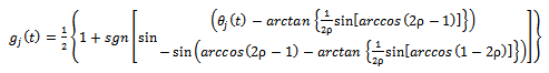 | (9) |
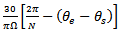
 end miller could undergo free flight or damped natural vibration when the radial immersion gets too low. The condition for this to occur becomes
 | (10) |
 as
as  while for down end-milling
  . If these angles are put into the inequality (10), the restriction on radial immersion
  for damped natural vibration for both Up end-milling and down end-milling becomes
 | (11) |
 evidently becomes given as
 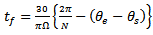 . The ratio of time interval of free flight to discrete delay becomes
 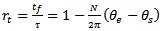 . If the start and end angles are put into this expression for
  the equations describing
  for Up end-milling and down end-milling respectively becomes equations (12) and (13)
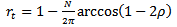 | (12) |
 | (13) |
 -component of cutting force for the tool becomes given as
 | (14) |
 tooth
tooth  as indicated in figure 4 is given by the non-linear law[4]
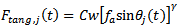 | (15) |
 is depth of cut,
  is the cutting coefficient associated with the workpiece material,
  is the actual feed and
  is an exponent that is not greater than one, having a value of
  for the three-quarter rule. The empirical relationship connecting the milling tangential and normal cutting forces shown in figure 4 is written in[4] to be seen in the works of Balint, Bali and Tlusty to have the form
 | (16) |
 is the difference between present and one period delayed position of tool, thus
 | (17) |
 | (18) |
 periodic function since tool-workpiece disposition repeats after every time
  interval.Stationary milling is the needed ideal that can only occur when there are no perturbations. In stationary milling the actual feed
 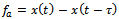 becomes equal to the prescribed feed per cutting period. That is,
  such that equation (18) becomes
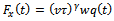 | (19) |
 -periodic like
  . For a milling process with the typical specification[5];
  (from the three-quarter rule), feed speed
 , a plot of periodic cutting force over interval of two periods is produced for both up end-milling and down end-milling at 0.5, 0.75 and 0.8 radial immersions as shown in figure6a, b and c respectively. It is seen that at each radial immersion
  has two different amplitudes, one above and other below the line
  The bigger amplitude of each periodic cutting force about zero value is of interest. The bigger the amplitude, the more likely the machined component will have tolerance error. At 0.5 radial immersion the cutting force amplitudes are 4.4 N and -2.7 N while they are 4.4 and 4.05 at 0.75 radial immersion for up end-milling and down end-milling respectively. Negative sign is retained to capture the meaning that cutting force is opposite to feed. At 0.8 radial immersion the cutting force amplitudes are 4.5 N and 4.15 N for up end-milling and down end-milling respectively. A plot of amplitude variation with
  is given in figure 7 in which is seen that up end-milling has higher amplitude than the down end-milling in the entire range of radial immersion. The conclusion drawn becomes that Though the Taylors’s tool life equation suggests equal longevity for up end-miller and down end-miller, the former is more damaging to tool than the latter since it generally has higher periodic cutting force amplitude. Reversal in direction of cutting force over a period exists for the down end-miller at low radial immersions since it has both positive and negative values when
  . This means that its vibratory motion occurs on both sides of the tool’s undisplaced equilibrium position. This is not the case for the up end-miller. It is seen that when
  , amplitude of stationary cutting force of interest for down end-milling becomes positive and approaches that of up end-milling as
  increases. It should be observed that cutting force varnishes over a time interval that is equal for both up end-milling and down end-milling. During this time interval which is given as
  for up end-milling and
 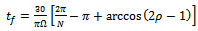 for down end-milling, the tool is not engaged with the workpiece thus in transient response.
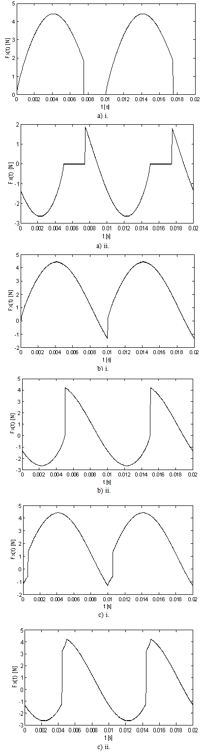 | Figure 6. Stationary Cutting Force Variation for a Three Tooth End-Milling At (A)  I. Up End-Milling, Ii. Down End-Milling I. Up End-Milling, Ii. Down End-Milling |
 | Figure 7. Amplitude of Stationary Cutting Force Variation Plotted Against Radial Immersion. Up End-Milling is Seen to Have Amplitude That is Fairly Invariant at about 4.4 N with  While Down End-Milling is Fairly Invariant At About -2.7 N Up To While Down End-Milling is Fairly Invariant At About -2.7 N Up To  |
3. Equation of Regenerative Vibration
- The parameters of the milling process as depicted on the dynamical model of figure 3 are;
 mass of tool,
  the equivalent viscous damping coefficient of the tool system and
  the stiffness of the tool system. These modal parameters could be extracted from plot of the tool frequency response function in a scheme of experimental modal analysis[6-8]. Figure 3 is a single degree of freedom vibration model of an end milling tool. Most encountered resonance in machining involves the fundamental natural frequency thus single degree of freedom vibration is satisfactory when it is well separated from the higher natural frequencies as seen in Stepan[9]. Chatter is an unstable vibration in machining due regenerative effects that are originally triggered by internal and external perturbations. Regenerative effect as seen in figure 3 is the effect of waviness created on a machined surface due to perturbed dynamic interaction between the tool and the workpiece. The present tool pass that is indicated as dashed curve has waviness that is not in phase with the last tool profile. A variation in chip thickness causes cutting force variation that results in vibration which subsequently builds up to chatter if cutting parameter combination is unfavourable.The free-body diagram for the tool dynamics shown in figure 3 is as depicted in figure 8.
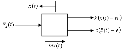 | Figure 8. Free-Body Diagram Of Tool Dynamics |
 | (20) |
 | (21) |
 , tool
  -periodic response
  due to periodic force of equation (19) and perturbation
  [4] then
 | (22) |
 | (23) |
 ), equation (23) simplifies to
 | (24) |
 | (25) |
 becomes
 | (26) |
 is the
  -periodic specific force variation. Equation (26) is re-written with the following compact notations;
  and
and  to give the periodic damped delayed differential equation of regenerative vibration of the system
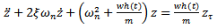 | (27) |
 and
and  made, equation (27) could be put in state differential equation form as
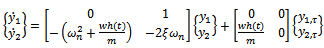 | (28) |
 and 2 . The natural frequency and damping ratio of the tool system are given in terms of modal parameters
  respectively as
  . These modal parameters are easily extracted from experimental plot of the tool frequency response function
  for forced single degree of freedom vibration. The damped natural vibration that occurs during the time interval
 obeys the ordinary differential equation
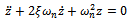 | (29) |
 . Putting the solution of form
  into equation (29) the characteristic equation becomes
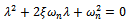 | (30) |
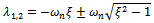 such that the transient response becomes
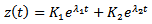 | (31) |
 and
and  , the constants become
 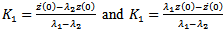 resulting in the response vector becoming
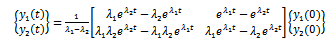 | (32) |
4. Time Finite Element Analysis of Chatter Stability
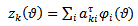
- Spatial finite element analysis is used for the estimation of quantities of interest at the nodes of discrete or quantized portions of a continuum. Among other fields of study this type of analysis is used in fluid mechanic to estimate property distribution[10], in vibration analysis to estimate; natural frequencies, mode shapes and forces[11, 12] and in structural analysis to estimate deflections. Ideas from Spatial finite element analysis are utilized for the so-called “time finite element analysis” (TFEA) also called “temporal finite element analysis or finite element in time”. TFEA has been variously in used in milling stability investigation[13-15]. Insperger et al[13] wrote that this method was first applied to an interrupted turning process by Halley and Bayly et al. They found that this method only yielded good result when the tool spends most of its cutting period in free flight. This shortcoming was corrected by Bayly et al when they used finer discretization. Stability of regenerative vibration using time finite elements involves dividing the period of cut into E time elements and estimating the perturbation motion of the system in each time element as a linear combination of trial functions. This process allows the formation of a discrete map that forms the substance of stability investigation. Within the present period of cut, the regenerative motion in the
 time element becomes
 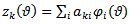 | (33) |
 | (34) |
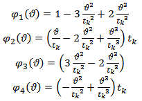 | (35) |
 is the local time of the
  time element of length
  . If uniform discretization is carried out then
  . Adopting uniform discretization, substitution of equations (33), (34) and (35) into equation (27) for the
  element gives an error of approximation
  as
as | (36) |
 element is set equal to zero giving
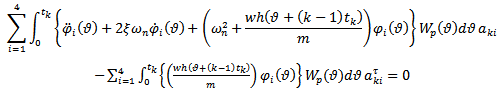 | (37) |
 as utilized in[13] are
 | (38) |
 element is seen from equations (33) and (35) taken together to give
 | (39) |
 | (40) |
 . Application of equation (32) gives that the state transition matrix
 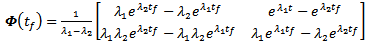 acts as a linear operator over a time interval
 transforming the end state
  of last element of delayed period of cut to the start state
  of the first element of present period of cut such that
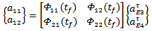 | (41) |
 independently into equation (37) enables the formation of a local matrix equation for each element which in light of the boundary conditions (40) and (41) are assembled into the global matrix equation of form
 | (42) |
 and
and  are
are  matrices. For example, if three elements are to be used, the global matrix equation becomes
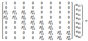
 where for the
  time element
 | (43a) |
 | (43b) |
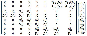
 is non-singular, the global matrix equation can be put in the form
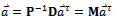 | (44) |
 -dimensional discrete time map of the system. It is seen that the nodal state vectors combine to form the global state vector of the discrete map. The matrix
  acts as a linear operator that transforms the delayed state
  to the present state
  . The matrix
  is called the monodromy matrix of the system. The nature of its eigenvalues also called characteristic multipliers determines the condition of stability of the system. The necessary and sufficient condition for asymptotic stability of the system is that each of the eigenvalues of the monodromy matrix has a magnitude that is less than one. In other words, all the eigen-values of the matrix
  must exist within a unit circle centred at the origin of the complex plane. Since the magnitude of the eigen-values depends on the cutting parameter combination, the parameter space of the system has to be demarcated into stable and unstable domains. This is achieved on the cutting parameter plane of spindle speed and depth of cut by tracking the stability transition curve along which the maximum magnitude characteristic multiplier lies on the unit circle. The two types of loss of stability (bifurcation) that are analytically and experimentally established for milling are[4] i. Period two or period doubling or flip bifurcation in which the exit of the unit circle of the critical characteristic multiplier
  is at
is at  .ii. Secondary Hopf or Neimark-Sacker bifurcation which involves a pair of complex conjugate characteristic multiplier leaving the unit circle.
 | Figure 9. (A) Flip Bifurcation (B) Secondary Hopf Bifurcation |
5. Results and Validation
- Making use of the relevant equations enables the eigen-value analysis of the monodromy matrix of reference system with specification;
 on the parameter plane of spindle speed
  and depth of cut
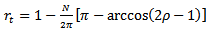
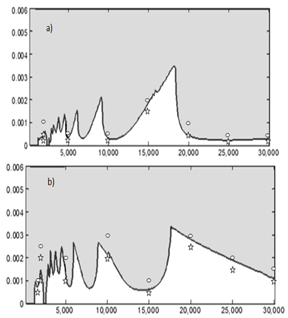
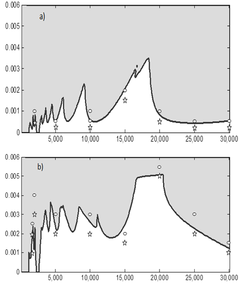
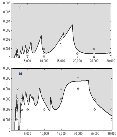
  leading to the stability charts of figures 10, 11 and 12 for 0.5, 0.75 and 0.8 radial immersions respectively. MATLAB contour command is utilized in the eigen-value analysis. Each of the stability charts is generated using 14 elements causing computation time per chart of a computer with processing speed of 2.10 Ghz to be about 2.92 hrs. The stable sub domain of each stability chart is left white while the unstable sub domain is filled dark.Though machine tools have a random pre-function (or history), stability information of a cutting parameter combination can still be fixed by assuming a constant pre-function since it is found that magnitude of such a pre-function has no effect on stability in large[5]. Making use of any constant history, equation (28) is solved using MATLAB dde23 at some chosen points of the stability charts. Stable MATLAB dde23 solutions exhibit decaying perturbation with time and are marked with star while the unstable ones exhibit growing perturbation with time and marked oval on the charts. Close agreement between the charts and MATLAB dde23 solutions attests to validity of the charts. For illustration some of the MATLAB dde23 solutions are presented in the form of phase trajectories as shown in figure 13. It is seen that stable trajectories (a, b and f of figure 13) collapse to zero motion with time evolution while the unstable ones (b, d and e of figure 13) diverge from initial condition
  .
. | Figure 10. Stability Charts At  with Stable Sub Domain Left White and the Unstable Sub Domain Filled Dark (A) Up End-Milling (B) Down End-Milling with Stable Sub Domain Left White and the Unstable Sub Domain Filled Dark (A) Up End-Milling (B) Down End-Milling |
 | Figure 11. Stability Charts At  =0.75 with Stable Sub Domain Left White and the Unstable Sub Domain Filled Dark (A) Up End-Milling (B) Down End-Milling =0.75 with Stable Sub Domain Left White and the Unstable Sub Domain Filled Dark (A) Up End-Milling (B) Down End-Milling |
 | Figure 12. Stability Charts at  =0.8 with Stable Sub Domain Left White and the unstable sub domain filled dark (a) up end-milling (b) down end-milling =0.8 with Stable Sub Domain Left White and the unstable sub domain filled dark (a) up end-milling (b) down end-milling |
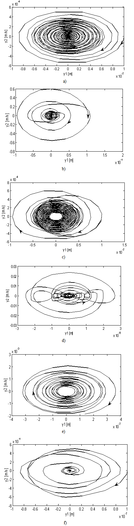 | Figure 13. SAMPLE PHASE TRAJECTORIES (a) UP END-MILLING AT  =0.5, =0.5,  =0.25 mm AND =0.25 mm AND  =5000 rpm (b) =5000 rpm (b)  =0.5, =0.5,  =3 mm AND =10000 rpm (c) =3 mm AND =10000 rpm (c)  =0.75, =0.75,  =1.5 mm AND =15000 rpm (d) =1.5 mm AND =15000 rpm (d)  =0.75, =0.75,  =5.5 mm AND =20000 rpm (e) =5.5 mm AND =20000 rpm (e)  =0.8, =0.8,  =0.5 mm AND =0.5 mm AND  =25000 rpm (f) =25000 rpm (f)  =0.8, =0.8,  =1 mm AND =1 mm AND  =30000 rpm =30000 rpm |
6. Discussions
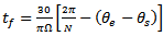
- It is seen that the down end-milling mode is more stable than the up end-milling mode. To quantify the superiority of chatter stability of down end-milling over up end-milling, numerical integration means such as trapezoidal or Simpson’s rule is utilized to approximate the area under each stability transition curve. The Simpson’s rule[16, 17] to estimate the area of stable subspace of each of the stability charts is
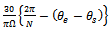
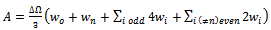 | (45) |
 is the steps of spindle speed,
  is an even number into which the stable area is divided and
  are the mesh points.
  . Making use of
  in equation (45), an estimation of stable area of the charts is as summarized in table1. It is seen from table1 that for the radial immersions considered, up end-milling operations are much less stable than the down end-milling operations. Switching from up end-milling mode to down end-milling mode at 0.5 radial immersion almost doubles the possibility of chatter free milling in the spindle speed range
  while at 0.75 and 0.8 radial immersions, this possibility almost triples in the same spindle speed range. Since productivity is measured in terms of material removal rate, it is proportional to the product of depth of cut and radial immersion. This means that the down end-milling mode allows freer choice of very productive stable operation. It is already established that up end-milling operation is more damaging to tool than down end-milling operation since it generally has higher periodic cutting force amplitude over the whole radial immersion range. Thus it is strongly recommend that an end-milling operation at partial radial immersion is carried out in the down end-milling mode for better product quality and longevity of tool and machine structure.
 7. Conclusions
- End-milling at partial radial immersion is seen to have two distinct modes. One of the modes which dynamically looks like the conventional milling is called “up end-milling” while the other that dynamically resembles the climb milling is called “down end-milling”. It results from analysis of cutting force and chatter stability that the down end-milling mode is better favoured for workshop application than the up end-milling mode. This is because up-end-milling is considered to be more damaging to tool than the down end-milling since it generally has higher periodic cutting force amplitude. The superiority of chatter stability of down end-milling over up end-milling is quantified by making use of the Simpson’s rule to establish that switching from up end-milling mode to down end-milling mode at 0.5 radial immersion almost doubles the possibility of chatter free milling in the spindle speed range
 while at 0.75 and 0.8 radial immersions this possibility almost triples in the same spindle speed range. This result is in conformity with the age long recognition from workshop practices that climb milling operations are more stable than conventional milling operations. Validation of the resulting stability charts is conducted using MATLAB dde23 analysis of selected points on the parameter plane of spindle speed and depth of cut.
References
| [1] | Youssef, H. A. and El-Hofy, H., 2008, Machining Technology: Machine Tools and Operations, CRC Press Taylor &Francis Group, pp. |
| [2] | Joshi, P. H., 2007, Machine Tools Handbook: Design and Operation, Tata McGraw-Hill Publishing Company Limited, New Delhi, pp.40-41. |
| [3] | Miller, R. and Miller, M. R., Machine Shop Tools and Operations, All new 5th edi., Willey Publishing Inc., New York, pp.253-254. |
| [4] | Insperger, T., 2002, “Stability Analysis of Periodic Delay- Differential Equations Modelling Machine Tool Chatter,” PhD thesis, Budapest University of Technology and Economics. |
| [5] | Ozoegwu, C. G., 2011, “Chatter of Plastic Milling CNC Machine,” M. Eng thesis, Nnamdi Azikiwe University Awka. |
| [6] | Gatti, P. L., and Ferrari, V., 2003, Applied Structural and Mechanical Vibrations: Theory, methods and measuring instrumentation, Taylor & Francis e-Library. |
| [7] | He, J. and Fu, Z., 2001, Modal Analysis, Butterworth Heinemann, Oxford. |
| [8] | Rao, S. S., 2004, Mechanical Vibrations (4th ed.), Dorling Kindersley, India. |
| [9] | Stepan, G., 1998, Delay-differential Equation Models for Machine Tool Chatter: in Nonlinear Dynamics of Material Processing and Manufacturing, edited by F. C. Moon, John Wiley & Sons, New York, p. 165-192. |
| [10] | Ihueze, C. C. and Ofochebe, S. M., 2011, “Finite Design for Hydrodynamic Pressure on Immersed Moving Surfaces,” International Journal of Mechanics and Solids, 6(2), pp.115-128. |
| [11] | Ihueze, C. C., Onyechi, P. C., Aginam, H. and Ozoegwu, C. G., 2011, “Finite Design against Buckling of Structures under Continuous Harmonic Excitation,” International Journal of Applied Engineering Research, 6(12), pp.1445-1460. |
| [12] | Ihueze, C. C., Onyechi, P. C., Aginam, H. and Ozoegwu, C. G., 2011, “Design against Dynamic Failure of Structures with Beams and Columns under Excitation,” International Journal of Theoretical and Applied Mechanics, 6(2), pp.153-164 |
| [13] | Insperger, T., Mann, B.P., Stepan, G., and Bayly, P. V., 2003, “Stability of up-milling and down-milling, part 1: alternative analytical methods,” International Journal of Machine Tools & Manufacture, 43, pp.25–34. |
| [14] | Bobrenkov, O. A., Khasawneh, F. A., Butcher, E. A. and Mann, B. P., 2010, “Analysis of milling dynamics for simultaneously engaged cutting teeth,” Journal of Sound and Vibration, 329, pp.585–606. |
| [15] | Bayly, P.V., Schmitz, T. L., Stepan, G., Mann, B. P., Peters, D. A. and Insperger, T., 2002, “Effects of radial immersion and cutting direction on chatter instability in end-milling,” Proceedings of IMECE’02 2002 ASME International Mechanical Engineering Conference & Exhibition New Orleans, Louisiana, November 17-22. |
| [16] | Riley, K. F., Hobson, M. P. and Bence, S. J., 1999, Mathematical Methods for Physics and Engineering, Low Prize ed., Cambridge University Press, pp.185. |
| [17] | Jain, M. K., Iyengar, S. R. K. and Jain, R. K., 2007, Numerical Methods for Scientific and Engineering Computation, Fifth ed., New Age International (P) Limited Publishers, pp.352 and 357. |