-
Paper Information
- Next Paper
- Previous Paper
- Paper Submission
-
Journal Information
- About This Journal
- Editorial Board
- Current Issue
- Archive
- Author Guidelines
- Contact Us
Applied Mathematics
p-ISSN: 2163-1409 e-ISSN: 2163-1425
2012; 2(4): 131-135
doi: 10.5923/j.am.20120204.06
The Numerical Solution of Heat Problem Using Cubic B-Splines
 Abstract
 Reference
 Full-Text PDF
 Full-Text HTML
Duygu Dönmez Demir , Necdet Bildik
Department of Mathematics, Faculty of Art and Science, Celal Bayar University, Manisa 45047, Turkey
Correspondence to: Duygu Dönmez Demir , Department of Mathematics, Faculty of Art and Science, Celal Bayar University, Manisa 45047, Turkey.
| Email: |  |
Copyright © 2012 Scientific & Academic Publishing. All Rights Reserved.
This paper discusses solving one of the important equations in Physics; which is the one-dimensional heat equation. For that purpose, we use cubic B-spline finite elements within a Collocation method. The scheme of the method is presented and the stability analysis is investigated by considering Fourier stability method. On the other hand, a comparative study between the numerical and the analytic solution is illustrated by the figure and the tables. The results demonstrate the reliability and the efficiency of the method.
Keywords: Cubic B-splines Finite Element Method, Collocation Method, Cubic B-splines, Finite Element Method
Article Outline
1. Introduction
- Consider the one dimensional initial-boundary value problem
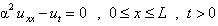 | (1) |
 | (2) |
 | (3) |
 along the rod where the coefficient
  is the thermal diffusivity of the rod and L is the length of the rod[5]. In this model, the flow of the heat in one-dimension that is insulated everywhere except at the two end points. Solutions of this equation are functions of the state along the rod and the time t. In the past, this problem has been widely worked over a number of years by numerous authors. But it is still an interesting problem since many physical phenomena can be formulated into PDEs with boundary conditions. The heat equation is of fundamental importance in diverse scientific fields. It is the prototypical parabolic partial differential equation in mathematics. In probability theory, the heat equation is connected with the study of Brownian motion via the Fokker–Planck equation[6]. Numerical solutions of those equations are very useful to study physical phenomena. One of the linear evolution equation which we deal with the numerical solution is the heat equation[7]. In 1946, Schoenberg first proposed the theory of B-splines[4]. Recurrence relations for the purpose of computing coefficients are given by Cox and de Boor[8,9]. The cubic B-splines collocation method was developed for Burgers’ equation and used for the numerical solution of the differential equations in[10,11]. Recently, spline function theory has been extended and developed to solve the differential equations numerically by various papers[12-14]. Furthermore some extraordinary problems has been numerically investigated by finite element methods such as Galerkin method, least square method and collocation method with quadratic, cubic, quintic and septic B-splines [15-17]. Various techniques of both the cubic spline and cubic B-spline collocation methods and their application have been developed to obtain the numerical solution of the differential equations. They possess some of advantages and are worth on using in the numerical techniques. So cubic spline collocation procedures exhibits the following the desirable features: (1) obtained governing system is always diagonal which permits easy algorithms; (2) it provides low computer cost and easy problem formulation. The requirement of the continuity up to the second degree are guaranteed at the mesh points over the domain and the first and second degree of the derivatives are directly evaluated[7,12,18].In this study the cubic B-splines collocation method is used for solving the heat equation (1) subject to (2) and (3) and the solutions are compared with the exact solution[19]. For constructing the cubic B-splines finite element method, we use collocation techniques as it was extensively used in[7,20,21]. In the section two, proposed method is presented and it is also given how to apply the collocation method with cubic B-splines finite element technique. In the section three, the stability analysis is investigated considering Fourier stability method. Finally, the numerical results and the related tables are given in the next section.
2. Collocation Method
- Let us consider the domain
 that is equally-divided with nodal points
  such that
 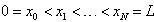 , i.e., finite elements of length
  for
for  , and also suppose that
  to be cubic B-splines at the nodal points
  for
for  . Using cubic B-splines
  , the exact solution
  is approached by an approximation
  such that
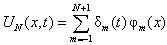 | (4) |
 is parameter in terms of the time t for
 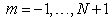 to be identified by the boundary conditions and the collocation conditions. The cubic B-splines
  are defined in[19].
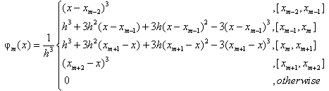 | (5) |
 defined in (5), the required values of
  and its first and the second derivatives with respect to x at the nodal points
  are identified in terms of
  as
as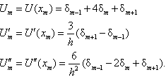 | (6) |
 , and
, and  in (1) and (2), respectively. Therefore the problem (1) subject to (2) and (3) is become
  | (7) |
 | (8) |
 | (9) |
 | (10) |
 | (11) |
 | (12) |
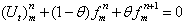
 is a parameter that when it takes the value 0, the scheme is so called forward Euler and also if
  , then the scheme is called Crank-Nicholson, and if
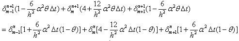
  , the scheme is so called backward Euler. Then we discretize the time derivative by means of finite difference so we have
 | (13) |
 , which has
  difference equations with
  unknown values as
 | (14) |
 Then this set of equations is a recurrence relationship of element parameters vector
  . Using the boundary conditions (9) and eliminating the parameters
  in (14), then the system may be rewritten as
 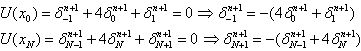 | (15) |
 unknown at each level of the time n in order to solve it using by Thomas algorithm.
 3. The Stability Analysis
- Now, the stability analysis is investigated by using very useful technique which is called Fourier stability method. Additionally the stability analysis is also used for various finite difference methods[22]. Considering the equation (13) and (14) together, then
 | (16) |
 | (17) |
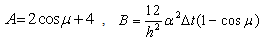
 may be written where
  , h is the step size defined in Section 2 and
  . By this equality, (17) can be reduced as
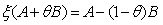 | (18) |
 . Then the solution is stable for
  using the Equation (14), since the inequality
  holds by the Fourier stability method.
4. Numerical Results and Discussion
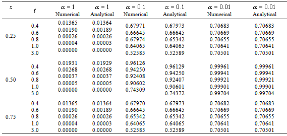
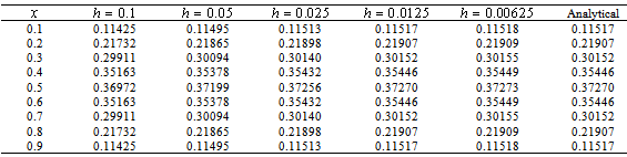
- In this section, we applied the method in Section 2 to problem (7) with (8) and (9) in order to solve it numerically. Since than numerical results are obtained. In order to control the validity and efficiency of the numerical solutions of the equation (7) in the domain [0,1] under the initial condition (2) and the boundary conditions (3), we calculated the analytical solution of the equation (7) with the initial and boundary conditions. Here, the time step is taken as
 in calculations. Mainly, Table 1 shows the both numerical solutions for some
  and the analytical solutions to comparing with the data for some values of t . It is seen from table that the method with decreasing step size gives better approximate solutions than the others.
|
 when
when  and
and 
 is taken in calculations with
  , the results are shown and compared for different values of h in Table 2. It is also seen from the table that the results calculated for
  , and
, and  coincide with the exact solution, while those for
  , are approached rapidly to the exact solutions.
|
 .
.5. Conclusions
- In this paper, we apply the collocation method with cubic B-splines finite elements to the heat equation successfully. In section 3, the stability of this method is analyzed considering Fourier stability method and it is found that the method is stable for
 . The results of the numerical solutions in Section 2 confirm that the accuracy, reliability and efficiency of the presented method which is applied in order to solve this type of the problem.