1. Introduction

Diseases can be transmitted many ways, some of which can be classified as either horizontal or vertical. In the case of HIV/AIDS, horizontal transmission can result from direct physical contact between an infected individual and a susceptible individual. Vertical transmission, on the other hand, can result from direct transfer of a disease from an infected mother to an unborn or newborn offspring. Diseases that can be transmitted vertically include chagas, dengue fever, hepatitis B and HIV/AIDS just to name a few. Vertical transmission of HIV/AIDS can occur during pregnancy, delivery or breastfeeding and is influenced by many factors, including maternal viral load and the type of delivery[1]. According to[2] and[3], about 20% of the children infected with HIV develop AIDS in the first year of their lives, and most of them die by the age of 4 years. The others, up to 80% of infected children, develop symptoms of HIV/AIDS at school entry age (7-9 years) or even during adolescence.

HIV/AIDS transmission in Africa is primarily through heterosexual sex and vertical transmission (mother-to-child). Forty percent of all HIV/AIDS cases result from mother to child transmission[4]. Fewer than 300 infants in the U.S acquired HIV through vertical transmission in 1997. In sub-Saharan Africa over 2.5 million children under the age of 15 have died of AIDS. Most of these children wereexposed to HIV during labour or breastfeeding. HIV/AIDS is globally a serious threat to future development

The impact of vertical transmission of HIV/AIDS has been felt mainly in Africa[1], where the level of literacy is low, the poverty level is very high and the quality of health services is generally very poor. A number of studies involving treatment of HIV-infected pregnant mothers (in Abidjan[5], and Thailand[6]) have shown that when HIV -infected mothers are treated with AZT (Zidovudine) and Nevirapine, the number of babies born infected is reduced significantly. Other studies[6, 7, 8] involving treatment of HIV-infected children have demonstrated further that effective treatment for these children can prolong their survival and significantly improve the quality of their lives. The current antiretroviral drugs (ARV) are known[9] to be effective in lowering viral loads, and the infected children may as a result reach adulthood and become sexually active.[10] studied a mathematical model on the dynamics of HIV/AIDS epidemic with vertical transmission.[11] proposed an HIV/AIDS model with vertical transmission and the period of sexual maturity of infected newborns which is incorporated in the model as a time delay.[12] proposed a model on the scope of the HIV/AIDS epidemic generally, and two of the major modes of transmission (mother–to–child and heterosexual intercourse) with respect to population distributions (0 – 5) years and 15 years and above.

In this study, we extend the model by[10], who considered vertical transmission of HIV/AIDS without treatment.[10] assumed that no juveniles born infected with HIV/AIDS lived long enough to reach the adolescent stage. This assumption was justified in 1991, since antiretroviral drugs capable of prolonging lives up to adulthood were unknown or not widely available. Using models which assumeconstant total population in arriving at or in assessing theeffectiveness of public health policies aimed at the control of such epidemics may fail to capture the severity of the epidemic in populations which are undergoing demographic changes. In this paper it is therefore intended to extend the work of[10] so as to incorporate treatment. Therefore we study and analyse the dynamics of HIV/AIDS with treatment and vertical transmission. Consequently, we formulate anon -linear system of differential equations that models the dynamics of transmission in a varying population. Models of HIV/AIDS dynamics that ignore the impact of vertical transmission, particularly during the current high usage of antiretroviral drugs, may fail to capture the actual impact of HIV/AIDS in a population.

2. Model Formulation

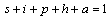
A non linear mathematical model is proposed and analyzed to study dynamics of HIV/AIDS with treatment and vertical transmission. In modelling the dynamics, the population of size at time with constant inflow of susceptible with rate where is the rate of recruitment into susceptible population is divided into five groups: Susceptibles , infectives (also assumed to be infectious), pre-AIDS patients , treated class and AIDS patients with natural mortality rate in all classes.

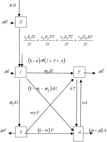Figure 2.1. Flow diagram of the model

The interaction between the classes will be assumed as follows: the susceptibles become HIV infected via sexual contacts with infectives which may also lead to the birth of infected children. A fraction of new born children are infected during birth and hence are directly recruited into the infective class with a rate and others die effectively at birth where is the fraction of newborns infected with HIV who dies immediately after birth and is the rate of newborns infected with HIV. We do not consider direct recruitment of the infected persons but by vertical transmission only.

It is also assumed that some of the infectives join the pre-AIDS class, depending on the viral counts, with a rate where is the rate of movement from infectious class and is the fraction of joining the pre-AIDS class. They then proceed with a rate to develop full blown AIDS. Some of the infectives proceed to join the treated class with a rate where is the fraction of joining treated class and then proceed with a rate to develop full blown AIDS while others with serious infection directly join the AIDS class with a rate . A Fraction of is assumed to get treatment. Taking into account the above considerations, we then have the following schematic flow diagram

It is also assumed that some of the infectives join the pre-AIDS class, depending on the viral counts, with a rate where is the rate of movement from infectious class and is the fraction of joining the pre-AIDS class. They then proceed with a rate to develop full blown AIDS. Some of the infectives proceed to join the treated class with a rate where is the fraction of joining treated class and then proceed with a rate to develop full blown AIDS while others with serious infection directly join the AIDS class with a rate . A Fraction of is assumed to get treatment. Taking into account the above considerations, we then have the following schematic flow diagram

The model is thus governed by the following system of non linear ordinary differential equations:

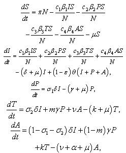(1)

where

are the sexual contact rates

is the average number of sexual partners per unit time

is the disease induced death rate in the AIDS patients class

is the rate at which AIDS patients get treatment

The initial conditions are taken as

and

To simplify the model, it is reasonable to assume that the AIDS patients and those in pre-AIDS class are isolated and sexually inactive and hence they are not capable of producing children i.e. 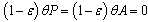and also they do not contribute to viral transmission horizontally i.e. and are negligible[1].

In view of the above assumptions, the system reduces to

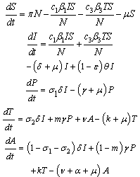(2)

The total population at any time is given by

.

This gives

We note that in the absence of the disease and infectives, the total population size is stationary for , declines for and grows exponentially for . So we shall assume that mortality rate , will be a function of state variables. Since the model is homogeneous of degree one, the variables can be normalized by setting , . This leads to the normalized system

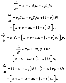(3)

where

and.

Continuity of right-hand side of the system (3) and its derivative imply that the model is well posed for .

3. Model Analysis

The nonlinear system (1) will be qualitatively analyzed so as to find the conditions for existence and stability of disease free equilibrium points[13]. Analysis of the model allows us to determine the impact of treatment and vertical transmission on the transmission of HIV/AIDS infection in a population. Also on finding the reproductive number, one can determine if the disease become endemic in a population or not.

3.1. Positivity of Solutions

It is necessary to prove that all solutions of system (3) with positive initial data will remain positive for all times . This will be established by the following theorem.

Theorem 1

Let . Then the solutions of the system (3) are positive .

Proof

From the first equation of the system (3), we obtain the inequality expression

(4)

As we obtain . Hence all feasible solution of system (3) enter the region 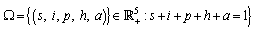. Similar proofs can be established for the positivity of .

3.2. Disease Free Equilibrium (DFE)

The disease free equilibrium of the normalized model (3) is obtained by setting

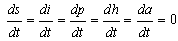(5)

At disease free equilibrium we have , and the system (3) becomes

Therefore the disease free equilibrium (DFE) denoted by of the system (3) is given by

(6)

3.3. Local Stability of DFE

The disease free equilibrium of the model (3) was given by

(7)

3.4. Model Reproduction Number

In order to assess the local stability of the established by the next generation method on the system (3), computation of the basic reproduction number is essential. The basic reproduction number is defined as the effective number of secondary infections caused by typical infected individual during his entire period of infectiousness[14]. This definition is given for the models that represent the spreading of infection in a population. It is obtained by taking the largest (dominant) eigenvalue (spectral radius) of

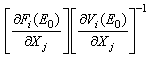(8)

where

is the rate of appearance of new infection in compartment ,

is the transfer of individuals out of the compartment by all other means,

is the disease free equilibrium.

By linearization approach, the associated matrix at disease free equilibrium is obtained as

It can be shown that the Eigen values of are .

where

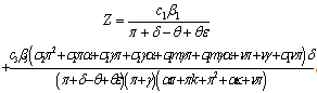(9)

It follows that the basic reproduction number for the normalised model system (3) with treatment and vertical transmission is given by

(10)

The disease free equilibrium of the treatment model system (3) with infective immigrants is locally asymptotically stable if and unstable if ,

Remark: It is noted that with high , which is a function of the number of sexual partners C , the number of invectives will increase which in turn increases the AIDS patients population. Thus in order to keep the spread of the disease at minimum, the number of sexual partners should be restricted.

3.5. The Endemic Equilibrium

To obtain an endemic equilibrium , we set each equation in the model (3) equal to zero. Solving the system while expressing each equilibrium point in terms of at steady state, we get 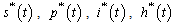, and as an endemic equilibrium point. Thus

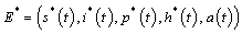is an endemic equilibrium where

with

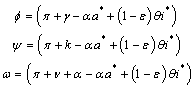and

We note that are always positive and this will happen if and only if . The model also exhibits a forward bifurcation for some estimated parameters as seen in figure 3.1 below:

A Forward or Transcritical bifurcation at the stationary solutions occurs at . If no biologically meaningful endemic stationary solution exists, and the disease free stationary solution is a global attractor. But if, the endemic solution exists and it is a global attractor, while the disease free solution is a saddle point. This is referred to as a forward bifurcation because in the neighbourhood of the bifurcation point, the endemic disease prevalence is an increasing function of

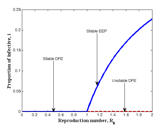Figure 3.1. Forward Bifurcation of the model (3)

3.6. Global Stability of the Endemic Equilibrium

Theorem 2

If , the endemic equilibrium of the model (3) is globally asymptotically stable.

Proof

To establish the global stability of the endemic equilibrium , we construct the following Lyapunov function:

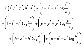By direct calculation of the derivative of along the solution of (3) we obtain

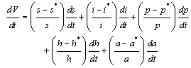(11)

which gives

where

and

Therefore from (11), if then, will be negative definite, implying that . Also , if and only if and . Therefore, the largest compact invariant set in 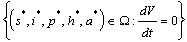is the singleton , where is endemic equilibrium of the normalized model system (3). By LaSalle’s invariant principle, it then implies that is globally asymptotically stable in if .

4. Numerical Simulations of the Model

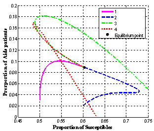
In order to verify the theoretical predictions of the model, the numerical simulations of the model (3) are carried out using the following set of estimated parameter values:

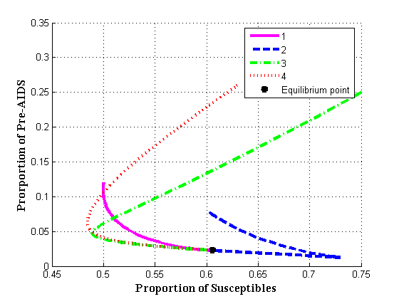
The endemic equilibrium values for and versus susceptibles are computed and shown graphically in figures 4.1(a) - 4.1(d)

The equilibrium points of the endemic equilibrium was obtained as

It is observed that for any starting initial value, the solution curves tend to the equilibrium point . Therefore it can be concluded that the system (3) is globally stable about this endemic equilibrium point for the estimated parameters.

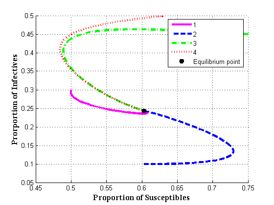Figure 4.1(a). Endemic equilibrium of proportion of infectives Vs Susceptibles

Figure 4.1(b). Endemic equilibrium of proportion of Pre-AIDS population

Figure 4.1(c). Endemic equilibrium of proportion of treated class

Figure 4.1(d). Endemic equilibrium of proportion of AIDS population

Figure 4.2(a) shows the distribution of proportion of population with time in different classes with neither new infected children into the population nor recruitments i.e. and .

It is seen that in the absence of vertical transmission into the community, the proportion of susceptible population decreases continuously resulting in the increase of the proportion of infective population initially but then decreases as all infectives subsequently develop full blown AIDS and the die naturally or by disease-induced deaths.

Figure 4.2(b) shows the variation of proportion of population in all classes with both recruitment of susceptibles and fraction of new born children which are infected at birth.

From figure 4.2(b) it can be seen that susceptibles first decrease with time. After undergoing ARV treatment their lives time are prolonged and thus their number increase reaching an equilibrium point.

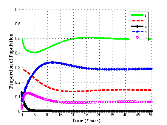Figure 4.2(b). Variation of population in different classes for and

Figures 4.3(a) - 4.3(c) below show the role of vertical transmission in the model i.e. the rate of recruitment of infected children directly into infective class is explicitly shown in

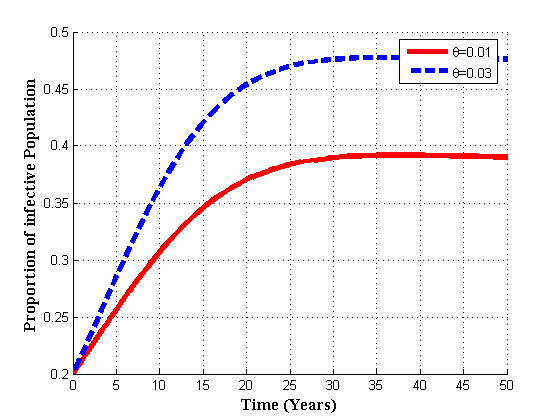Figure 4.3(a). Variation of infected population for different values of

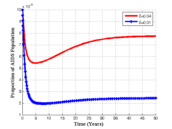
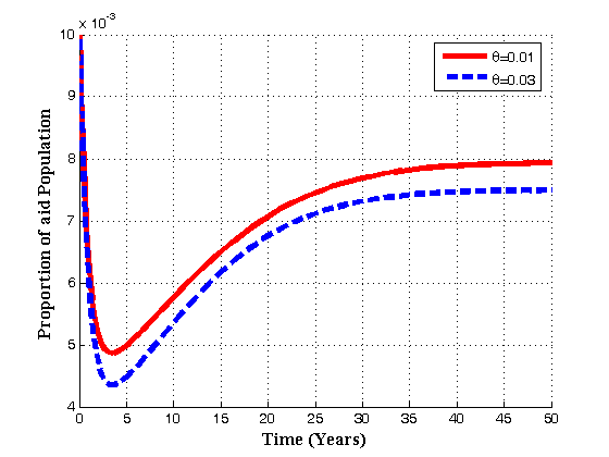Figure 4.3(b). Variation of AIDS population for different values of

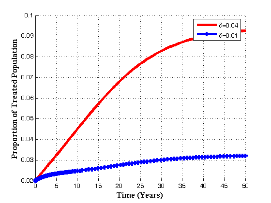
Figure 4.3(c). Variation of Treated class for different values of

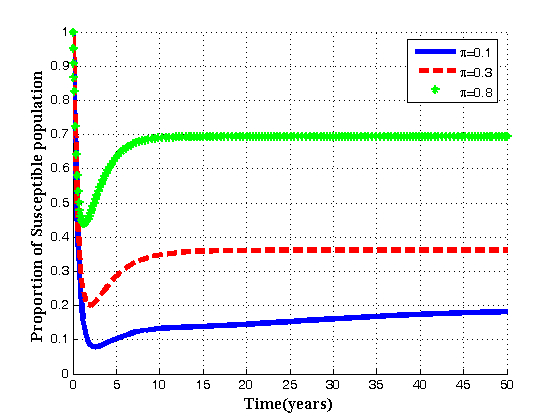Figure 4.4(a). Variation of Susceptibles for different values of

It is seen that in figure 4.3(a) that as the rate of infected born children increase, the proportion of infective population also increases. In figure 4.3(b) it is seen that if the value of is increased, the proportion of AIDS population decrease with time and then increase until it reach its equilibrium position. Thus if infected born children are intervened by treatment, the overall infective population will remain under control thus reducing the AIDS population. In 4.3(c) it is seen that as the rate of infected born children increase, the treated population decrease.

Figures 4.4(a) – 4.4(c) below show the impact of recruitment rate for susceptibles, treated class and AIDS patients for different values of

It is seen that for different values of , as recruitment rate increase, the susceptible population also increase. While the inflow of susceptible increase, the treated population and AIDS population decrease with time until they reach equilibrium due to treatment.

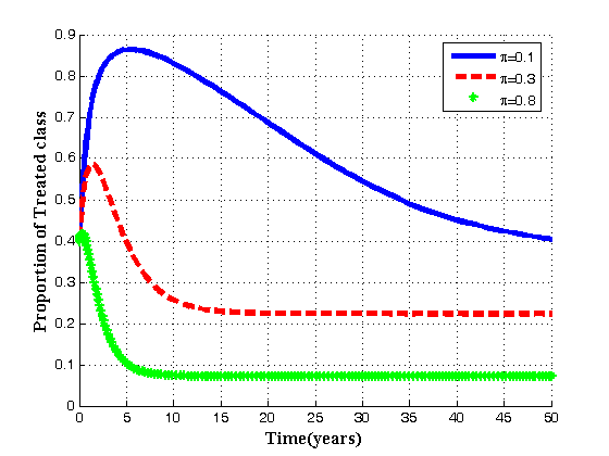Figure 4.4(b). Variation of Treated population for different values of

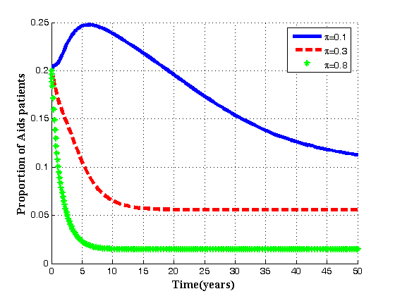Figure 4.4(c). Variation of AIDS population for different values of

Figures 4.5(a) – 4.5(d) depict the variation of infectives, pre-AIDS, Treatment and AIDS population respectively with time for different values of movement rate of individuals from infective class to pre-AIDS, Treatment or AIDS depending upon the viral counts.

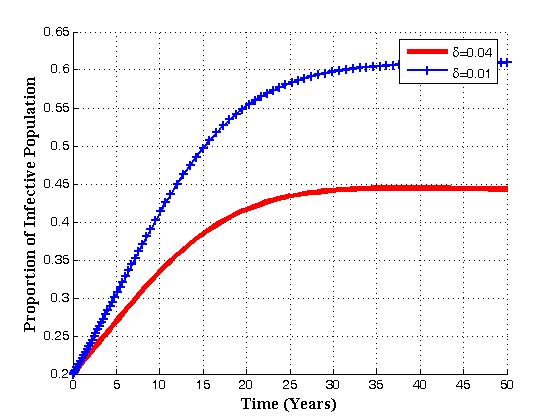Figure 4.5(a). Variation of Infective population for different values of

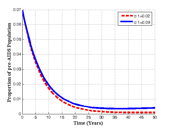
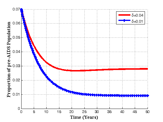Figure 4.5(b). Variation of pre-AIDS population for different values of

Figure 4.5(c). Variation of Treated class for different values of

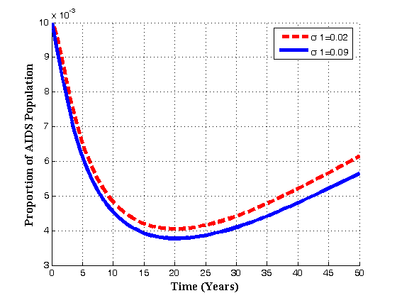
Figure 4.5(d). Variation of AIDS population for different values of

It is seen that with increase in the value of movement rate , the infected population decrease which in turn increase the treated population. Also with the increase of , the pre-AIDS and AIDS population decrease with time until they reach the equilibrium values.

Figures 4.6(a) – 4.6(d) shows the Variation of population in the classes with fraction of movement rate from infectious class.

Figure 4.6(a). Variation of pre-AIDS population for different values of

Figure 4.6(b). Variation of AIDS population for different values of

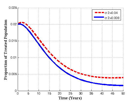Figure 4.6(c). Variation of Treated population for different values of

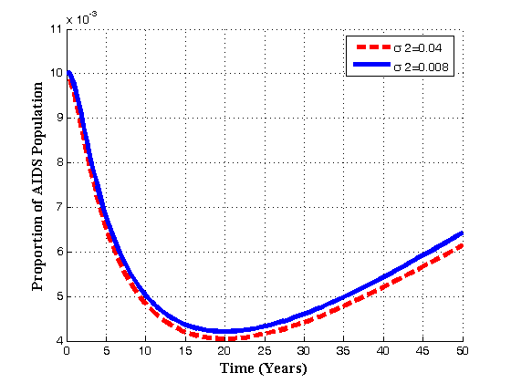Figure 4.6(d). Variation of AIDS population for different values of

It is seen that from the figures that when increases, the pre-AIDS population decrease continuously. It might be it is because of treatment to the patients. The case is different for the AIDS class. It can be seen that when increases, the AIDS population decrease with time it reaching equilibrium point and then increase with time. This is caused by ARVs treatment and its effect in prolonging the life span.. It can also be noted from the graph that, as increases treated population initially increase. As time progress, it decrease, but the AIDS patients population decrease continuously reaching equilibrium and then increase implying that the disease still exist.

Figures 4.7(a) – 4.7(d) predict the variation of the contact rates of susceptibles with respect to infectives and susceptibles with respect to treated class in the susceptibles and infectives classes.

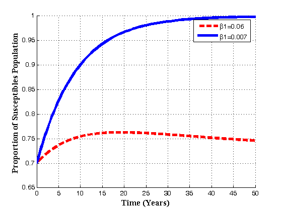Figure 4.7(a). Variation of susceptibles population for different values of

Figure 4.7(b). Variation of infectives population for different values of

Figure 4.7(c). Variation of susceptibles population for different values of

Figure 4.7(d). Variation of infectives population for different values of

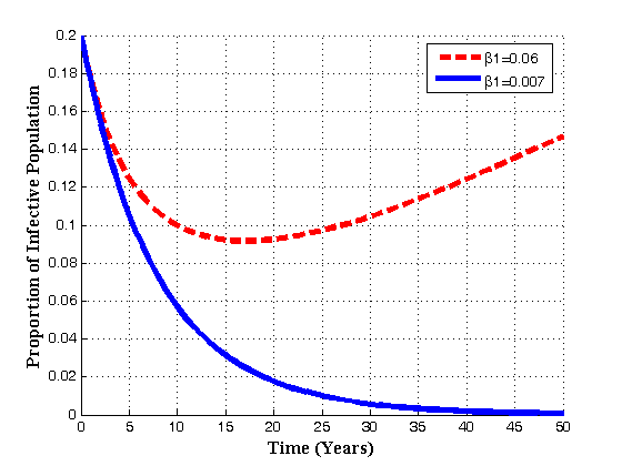
The graphs show that as the contact rate increases, the susceptibles decrease, infectives class decrease implying that treatment increase. Also as the contact rates of susceptible with treated population increase the susceptible initially increase with time and then it reaches its equilibrium point. But it is differerent to infectives as increases. The infectives decrease with time reaching its equilibrium point and then increase again.

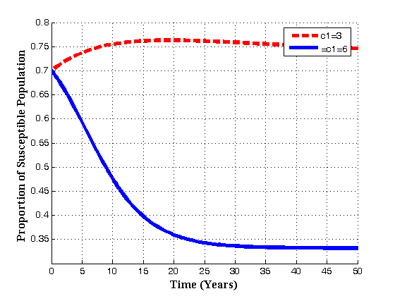
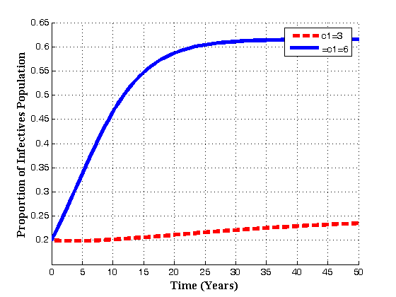
Figures 4.8(a) – 4.8(b) below show the variation of susceptibles and infectives population for different values of number of sexual partners of susceptibles with infectives , and between susceptibles with treated population .

Figure 4.8(a). Variation of Susceptibles population for different values of

Figure 4.8(b). Variation of Infectives population for different values of

Figure 4.8(c). Variation of Susceptibles population for different values of

Figure 4.8(d). Variation of Infectives population for different values of

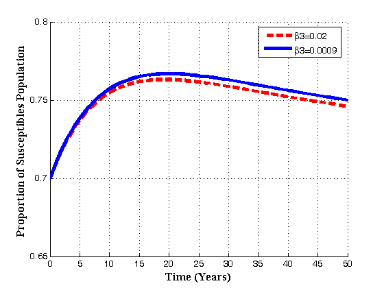
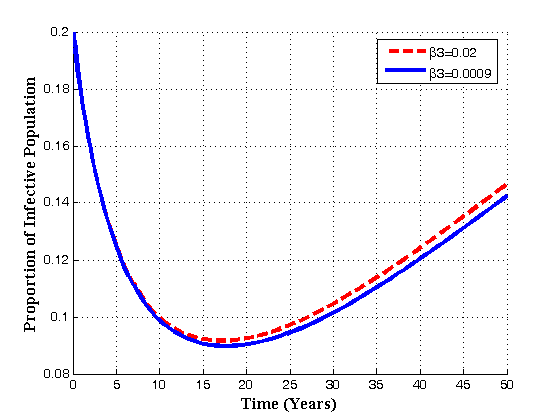
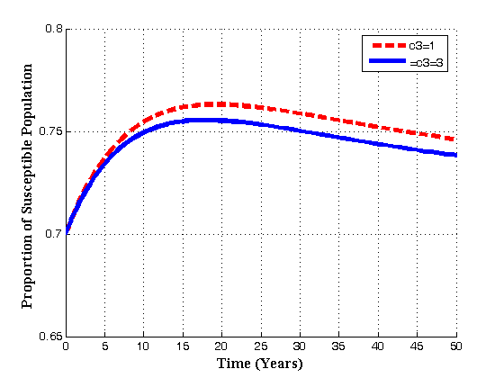
From the graphs, it is seen that as the number of sexual partners of susceptibles with infectives increases with time, susceptibles decreases continuously and infectives increases continuously. Also it is seen that if the number of sexual partners of susceptibles with treated population increases with time, susceptibles first increase and then decrease with time as shown in fig. 4.8(c) due to the loss of immunity. 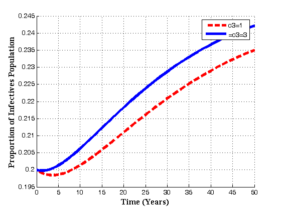But for infectives, it seen that as increases, the infectives also increase. Thus it can be concluded that, in order to reduce the spread of the disease, the number of sexual partners as well as unsafe sexual interaction with an infectives should be restricted.

Figures 4.9(a) and 4.9(b) shows the variation of treatment rates in treated class and AIDS population.

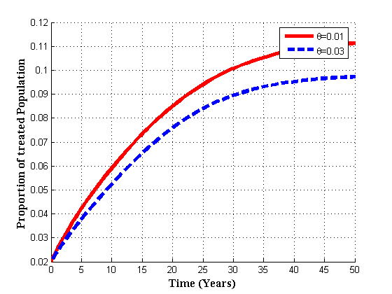
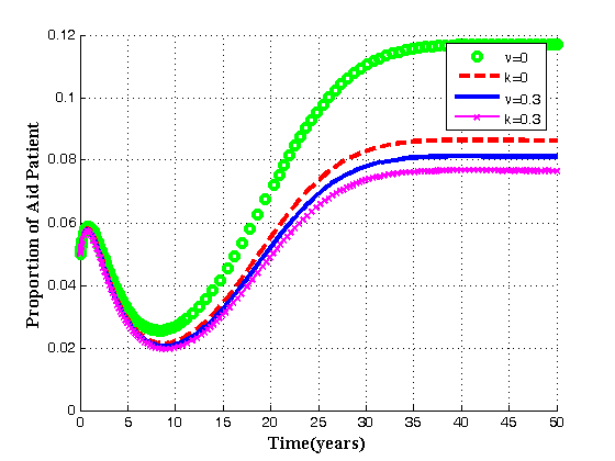Figure 4.9(a). Variation of AIDS patients for different values of and .

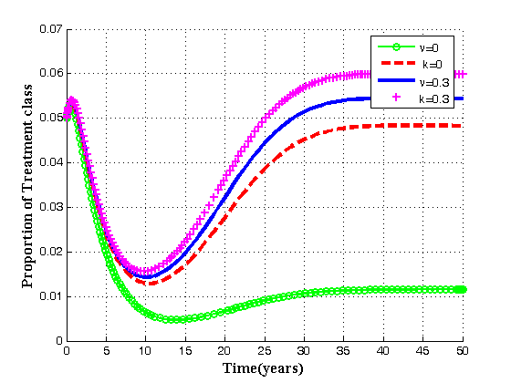Figure 4.9(a). Variation of treated patients for different values of and .

It is observed that if treatment rate is zero, the disease increase with time whereas treated population decrease. Also the graphs show that as the rates of treatment increase, the AIDS patients decrease due to treatment.

In figure 4.10 below, the effect of disease induced death rate is shown.

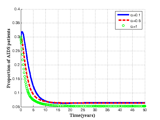Figure 4.10. Variation of AIDS populations for different values of .

It can be seen that as increases, the population of AIDS patients decrease. It is found that the AIDS induced death rate, can be controlled by ARVs strengthening health education regarding the AIDS disease. It can also be noted that the respective populations tend to the equilibrium level as time progresses. Hence the endemic equilibrium is globally asymptotically stable for the chosen set of parameter value.

5. Discussion and Conclusions

In this paper, a non-linear mathematical model to study the transmission of HIV/AIDS in a population of varying size with treatments and vertical transmission was proposed. Both qualitative and numerical analysis of the model was done. The model incorporates the assumption that due to sexual interaction of susceptibles with infectives, the infected babies born increase the growth of infective population directly. It was shown that there exists a feasible region where the model is well posed in which a unique disease free equilibrium point exists.

The disease free and endemic equilibrium points were obtained and their stabilities investigated. A numerical study of the model has been conducted to see the effect of certain key parameters on the spread of the disease. It was established that the disease-free equilibrium is locally asymptotically stable if the basic reproduction number and for it is unstable and the infection is persists in the population.

The endemic equilibrium, which exist only when , is always locally asymptotically stable. It is found that an increase in the rate of vertical transmission leads to the increase of the population of infectives which in turn increase the pre-AIDS and AIDS population. From the numerical simulation, it is shown that by controlling the rate of vertical transmission, the spread of the disease can be reduced significantly.