Rajan Arora, Sanjay Yadav
Indian Institute of Technology Roorkee, Saharanpur campus, Saharanpur, U.P.-247001, India
Correspondence to: Sanjay Yadav, Indian Institute of Technology Roorkee, Saharanpur campus, Saharanpur, U.P.-247001, India.
| Email: |  |
Copyright © 2012 Scientific & Academic Publishing. All Rights Reserved.
Abstract
In this paper, the exact traveling wave solutions of thegeneralized forms B(n, 1) and B(-n, 1) of Burgers’ equation are obtained by using (G`/G)-expansion method. It has been shown that the (G`/G)-expansion method, with the help of computation, provides a very effective and powerful tool for solving non-linear partial differential equations
Keywords:
(G`/G)-expansion Method, Generalized Forms B(N, 1) And B(-N, 1) of Burgers’ Equation, Traveling Wavesolutions, Exact Solutions
Cite this paper: Rajan Arora, Sanjay Yadav, Application of The (-Expansion Method For Solving The Generalized Forms B(n,1) andB(-n,1) of Burgers’ Equation, Applied Mathematics, Vol. 2 No. 3, 2012, pp. 66-69. doi: 10.5923/j.am.20120203.04.
1. Introduction
The study of non-linear partial differential equations plays a very important role in many fields of mathematics and physics such as fluid dynamics, plasma physics, astro physics, solid state physics and quantum field theory. To obtain the solutions of non-linear partial differential equations, many methods were used, such as the Similarity transformation method[6,10], Backlund transformation method[7], the sine-cosine method[3,4], the Jacobi elliptic function method[8], the tanh method[11-14], the exp-function method[9,17], the inverse scattering method[1], and so on. One of the most powerful and direct methods for constructing solutions of non-linear partial differential equations is the (G`/G)-expansion method[2,5,16]. This method is first introduced by Wang et al.[16], and it has been widely used for finding exact solutions of non-linear partial differential equations. In this method, the linearization of non-linear differential equations for traveling wave is performed with a certain substitution which leads to a.second-order differential equation with constant coefficients. The calculations are performed with a computer algebra system for finding solutions of the non-linear equations The generalized forms B(n,1) and B(-n,1) of Burgers’ equation[18] are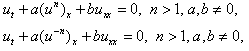 | (1) |
where the dependent variable is a function of space variable x and time variable t, a and b are arbitrary constants.The generalized forms of Burgers’ equation appear in various areas of mathematics, such as in the modeling of fluid dynamics, the propagation of waves, and traffic flow. Here, our goal is to obtain the exact traveling wave solutions for the generalized forms of Burgers’ equation by using (G`/G)-expansion method.
2.The (G`/G)-expansion Method
The (G`/G)-expansion method ([2,5,16]) is a powerful solution method for the computation of exact traveling wave solutions of partial differential equations (PDEs).We consider the non-linear PDE for  in the form:
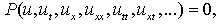 | (2) |
where is the unknown function depending on space variable X and time variable t, and p is a polynomial in
  and its partial derivatives, in which the highest orderderivatives and nonlinear terms are involved. To find the traveling wave solution of PDE (2), we introduce the variable
  so that
  , where
  is a constant. Based on this, we use the following changeof partial derivatives
 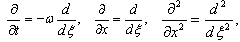 and so on for the other derivatives. Thus PDE (2) reduces to an ordinary differential equation (ODE)
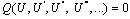 | (3) |
where the primes denote the derivative with respect to .Eq. (3) is then integrated as long as all terms contain derivatives, where integration constants are considered zeros.Now, we suppose that the solution of the ODE (3) can be expressed by apolynomialin
  )as follows:
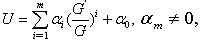 | (4) |
where satisfies the second order linear ODE in the form
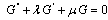 | (5) |
where  , and
, and  and
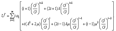
and  are real constants which are to be determined. Using (4) and (5), we obtain
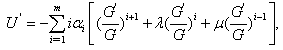 | (6) |
 | (7) |
Using the general solution of (5), we have for ,
,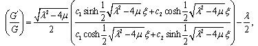 | (8) |
and for
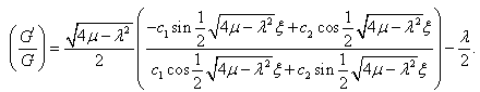 | (9) |
To determine U explicitly, we take the following four steps:Step 1. Determine the integer m by substituting (4) along with (5)into (3), and balancing the highest order nonlinear term(s) and the highest order partial derivative.Step 2. By substituting (4)and (5)into (3)with the value of m obtained in Step 1, and collecting all term(s) with the same order of together, the left-hand side of(3) converts into polynomial in
  . Then setting coefficients of
  to zero, we obtaina set of algebraic equations in
 .Step 3. Solve the system of algebraic equations obtained in step 2 for
  and
and  by use of Mathematica.Step 4. By substituting the results obtained in the above steps, we can obtain a series of fundamental solutions of (3).
3.Applications
In this section, we apply the (G`/G)-expansion method to construct the traveling wave solution of generalized forms of Burgers’ equation.
3.1 The B (n, 1) Burgers’ equation
This B(n, 1) Burgers’ equation is given as | (10) |
Using the transformation ,where
 , the PDE is reduced to an ODE
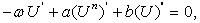 | (11) |
where primes denote the derivative with respect to  . Integrating once with respect to
  and taking constant of integration to be zero, (11) reduces to
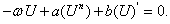 | (12) |
Now balancing and
and  , we obtainA necessary condition for obtaining a closed form analytic solution is that m must a positive integer. Using the transformation
  | (13) |
(12) converts to  | (14) |
Now, balancing  and
and  we obtain 2m=m+1 so
 .Writing the solution of (14) in the form
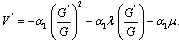
 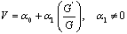 | (15) |
Using (4) and (15), we obtain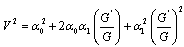 | (16) |
 | (17) |
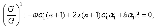
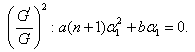
Substituting (15), (16) and (17) into (14), and setting the coefficients of  to zero, we obtain a system of algebraic equations in
  as follows:
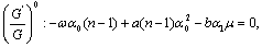 | (18) |
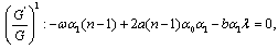 | (19) |
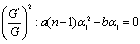 | (20) |
Solving the system of equations (18)-(20) by Mathematica, we obtain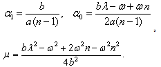 | (21) |
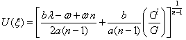
By using (21), the expression (15) can be written as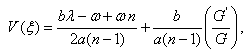 | (22) |
Where  is defined by (8) and (9). Nowusing
 | (23) |
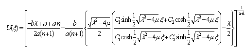
When  we obtain hyperbolic function solution of (10) as
 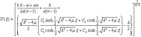 | (24) |
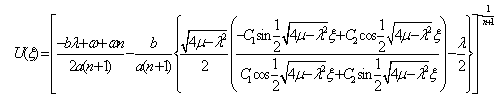
When  , we obtain trigonometric functionsolution of (10) as
 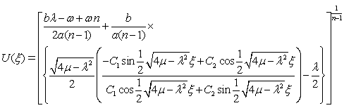 | (25) |
where,  and
and  and
and  are arbitrary constants and
 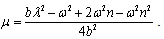 If we set
 in (24), then soliton solution of (10) is obtained as
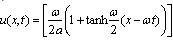 | (26) |
If we set
 in (24), then soliton solution of (10) is obtained as
 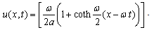 | (27) |
We see that (26) and (27) are the particular cases of the general exact solution (24). The solutions (26) and (27) are exactly same solutions as obtained by Wazwaz[18] for the above values of constants. Hence, our solutions (24) and (25) are more general.
3.2.The B(-n,1) Burgers’ equation
The B(-n,1) Burgers’ equation is | (28) |
Proceeding as earlier, we obtain theODE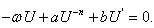 | (29) |
Now balancing  and
and  , we obtainNow using the transformation
  in (29), we obtain
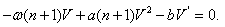 | (30) |
Now balancing  and
and  we obtain 2m=m+1so
 . Setting the coefficients of
  to zero, we obtain a system of algebraic equations in
  as follows:
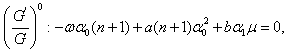 | (31) |
 | (32) |
 | (33) |
Solving the system of equations (31)-(33) by Mathematica, we obtain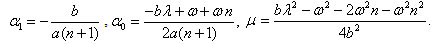 Where
Where  free parameter, now using
  , the solution of (28) is given by
 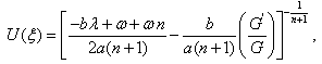 | (34) |
where is defined by (8) and (9).When
 | (35) |
When 
 | (36) |
where,  and
and  and
and are arbitrary constants and
 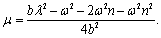 If we set
  and
and then (35) yields
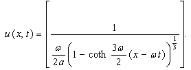 | (37) |
Similarly, if we set  and
and  then (35) yields
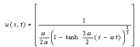 | (38) |
We observe that the solutions (37) and (38) obtained for Burgers’ equation (28) are particular cases of solution (35). These solutions are exactly same as the solutions obtained by Wazwaz[18] for the above values of constants.
4.Conclusions
In this paper, we used the (G`/G)-expansion method to obtain the exact traveling wave solutions of the generalized forms of Burgers’ equation. The solution method is very simple and effective, and the solutions are expressed in the form of hyperbolic functions and the trigonometric functions. It is shown that this method is a good tool for handling non-linear partial differential equations. Correctness of the solutions is also checked by comparing with the solutions obtained by Wazwaz[18], and substituting them back into the original equations with the help of Mathematica.
References
| [1] | Ablowitz,M.J. and Segur,H.(1981).Solitons and Inverse Scattering Transform. SIAM, Philadelphia. |
| [2] | Aslan,İ.(2009). Exact and explicit solutions to some nonlinear evolution equations by utilizing the ( G`/G)-expansion method. Appl. Math. Comput. 215, 857–863. |
| [3] | Borhanifar,A., JafariH.,andKarimi S.A.(2009). New solitary wave solutions for the bad Boussinesq and good Boussinesq equations, Numer. Methods for Partial Differential Equations 25 ,1231–1237. |
| [4] | Borhanifar, A.,Jafari,H. andKarimi,S.A. (2008). New solitons and periodic solutions for the Kadomtsev–Petviashvili equation. Nonlinear Sci. Appl. 4, 224–229. |
| [5] | Bekir A.(2008),Application of the ( G`/G)-expansion method for nonlinear evolution equations. Phys. Lett. A 372, 3400–3406. |
| [6] | Doyle, J., andEnglefield, M.J. ( 1990).Similarity Solutions of a Generalized Burgers Equation. IMA J. Applied Math. 44 ,145-153. |
| [7] | Karasu-KalcanliA.andSakovich.S.(2001). Bäcklund transformation and special solutions for the Drinfeld–Sokolev–Satsuma–Hirota system of coupled equations. J. Phys. A. Math. Gen. 34, 7355–7358. |
| [8] | Liu,G.T. and Fan,T.Y.(2005). New applications of developed Jacobi elliptic function expansion methods. Phys. Lett. A 345, 161–166. |
| [9] | Liu,G.T., Fan,T.Y.(2005). New applications of developed Jacobi elliptic function expansion methods. Phys. Lett. A 345, 161–166. |
| [10] | Miller, J.C., andBernoff, A.J.(2003).Rates of Convergence to Self-Similar Solutions of Burgers’ Equation. Studies in Applied Math. 111, 29-40. |
| [11] | Malfliet,W.,Hereman,W.(1996). The tanh method: exact solutions of nonlinear evolution and wave equations. Phys. Scr. 54, 563–568. |
| [12] | Malfliet,W.(1992). Solitary wave solutions of nonlinear wave equations. Am J Phy; 60(7), 650–658. |
| [13] | Malfliet,W.andHereman W.(1996). The tanh method: II. Perturbation technique for conservative systems.PhysScr; 54, 569–575. |
| [14] | Wazwaz,A.M.(2005). Exact solutions to the double sinh-Gordan equation by tanh method and avariable separated ode method. Compt.Math. Appl. 50,1685-1696. |
| [15] | Wang M.L.(1996). Exact solution for a compound KdV-Burgers equations. Phys. Lett. A 213, 279–287. |
| [16] | Wang,M.L. Li,. X. andZhang, J.(2008). The ( G`/G )-expansion method and traveling wave solutions of nonlinear evolution equations in mathematical. physics, Phys.Lett. A 372, 417–423. |
| [17] | Wen ,Y.X. Zhou, X.W. and He,J.H.(2008). Exp-function method to solve the nonlinear dispersive k(m, n) equations, Int. J. Nonlinear Sci. Numer. Simul. 9,301–306. |
| [18] | Wazwaz A.M.(2005).Travelling wave solutions of generalized forms of Burgers, Burgers-KDV and Burgers-Huxley equations. Appl.Math.Comput169, 639-656. |
 Abstract
 Reference
 Full-Text PDF
 Full-text HTML