-
Paper Information
- Next Paper
- Paper Submission
-
Journal Information
- About This Journal
- Editorial Board
- Current Issue
- Archive
- Author Guidelines
- Contact Us
Applied Mathematics
p-ISSN: 2163-1409 e-ISSN: 2163-1425
2012; 2(3): 58-65
doi: 10.5923/j.am.20120203.03
Solution of Magnetohydrodynamic Flow in a Rectangular Duct by Chebyshev Polynomial Method
 Abstract
 Reference
 Full-Text PDF
 Full-Text HTML
İbrahim Çelik
Faculty of Arts and Sciences, Department of Mathematics, Pamukkale University, Denizli, Turkey
Correspondence to: İbrahim Çelik , Faculty of Arts and Sciences, Department of Mathematics, Pamukkale University, Denizli, Turkey.
| Email: |  |
Copyright © 2012 Scientific & Academic Publishing. All Rights Reserved.
In this study, Chebyshev polynomial method is applied to solve magnetohydrodynamic (MHD) flow equations in a rectangular duct in the presence of transverse external oblique magnetic field. In present method, approximate solution is taken as truncated Chebyshev series. The MHD equations are decoupled first and then present method is used to solve for positive and negative Hartmann numbers. Numerical solutions of velocity and induced magnetic field are obtained for steady-state, fully developed, incompressible flow for a conducting fluid inside the duct. The results for velocity and induced magnetic field are visualized in terms of graphics for values of Hartmann numbers .
Keywords: Magnetohydrodynamic flow, Chebyshev series, Partial Differential Equation
Article Outline
1. Introduction
- Theoretical study of magnetohydrodynamic flow problems within the ducts are frequently encountered in cooling systems of nuclear reactors, magnetohydrodynamic (MHD) generators, blood flow measurements, pumps and accelerators. Due to coupling of the equations for electrodynamics and fluid mechanics, exact solutions are possible only for some simple situations. By using several numerical techniques such as Finite Difference Method (FDM), Finite Element Method (FEM), Finite Volume Method (FVM) and Boundary Element Method (BEM), approximate solutions for the MHD flow problems can be obtained.Singh and Lal[1-3] have used FDM and FEM to solve MHD flow for small Hartmann numbers M less then 10. Gardner and Gardner[4] used bi-cubic B-spline elements with FEM for Hartmann numbers less than 10. Tezer-Sezgin and Köksal[5] extended these studies to moderate Hartmann numbers up to 100 by using standard FEM with linear and quadratic elements. Further, Demendy and Nagy[6] have used the analytical finite element method to obtain numerical solution in the range of the Hartmann numbers M
 1000. Barreti[7] obtained FEM solution for the high values of M. However, he indicated a method which is computationally very memory intensive and therefore time consuming. Neslitürk and Tezer-Sezgin[8,9] solved MHD flow equations in rectangular ducts by using stabilized FEM with free bubble functions but their method is also time and memory consuming for large M numbers.The BEM applications for solving MHD duct flow arise from the difficulties for which the solutions of huge systems are obtained in FEM due to the domain discretization. Singh and Agawal[10], Tezer-Sezgin[11], Liu and Zhu[12], Tezer- Sezgin and Han Aydın[13], Carabineanu at al.[14] and Bozkaya and Tezer-Sezgin’s[15] papers are some of the publications on the BEM solutions of MHD duct flow problems for the small and moderate values of Hartmann numbers M
 . Bozkaya and Tezer-Sezgin employed the Dual Reciprocity Boundary Element Method (DRBEM) [15,16] for non-conducting walls and also time-domain BEM[17] for arbitrary wall conductivity unsteady MHD flow.To obtain velocity and induced magnetic field for the stady-state fully developed MHD flow for Hartmann numbers ranging from M=10 to 50, Tezer[18] has used Polynomial based Differential Quadrature (PDQ) and Fourier expansion based Differential Quadrature (FDQ) methods with equal and unequal spaced grid points.Dehghan and Mirzaei [20] have given the meshless local boundary integral equation (LBIE) method to obtain the numerical solution of the coupled equations in velocity and magnetic field for unsteady magnetohydrodynamic (MHD) flow through a pipe of rectangular and circular sections with non-conducting walls.Çelik [21] has represented Chebyshev Collocation Method for partial differential equation and applied to solve magnetohydrodynamic (MHD) flow equations in a rectangular duct in the presence of transverse external oblique magnetic field.Chebyshev series solution has been developed and applied to Linear Integro-Differential Equations by Koroglu[19]. Kesan[22] has been concerned with the Chebyshev polynomial solutions of the second-order linear partial differential equations.The aim of this paper is to use Chebyshev Polynomial Method for which approximate solution is taken as truncated Chebyshev series towards obtaining velocity and induced magnetic field for the steady-state oblique external magnetic field through a rectangular duct. The MHD equations were decoupled first and then were solved for positive and negative Hartmann numbers since the sign of Hartmann number was the difference in the decoupled equations. Chebyshev Polynomial Method has high potential as an alternative compared to the other solution techniques mentioned above with Hartmann numbers ranging from M=0 to1000
 2. Chebyshev Polynomial Method
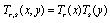
- Second order partial differential equations with variable coefficients may be expressed in the following form:
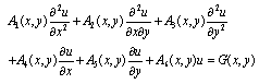 | (1) |
 and G are functions of x and y defined in the interval of
  . Any range
  can transformed into the basic range
  with the change of variables
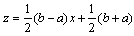 and
and 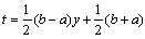 .Approximate solution of the above differential equation is expressed as the truncated Chebyshev series:
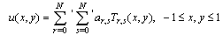 | (2) |
 ,
,  and
and  are the Chebyshev coefficients.
  denotes the Chebyshev polynomials of the first kind of degree r defined by The truncated Chebyshev series solution in (2) can be expressed in the matrix form as
 | (3) |
 and
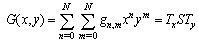
and 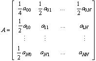 To obtain the solution of Eq. (1) in the form (3), first, Eq. (1) must be reduced to a differential equation whose coefficients are polynomials. For this aim, it is assumed that the functions
  and G can be expressed in the forms
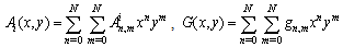 ,Hence, Eq. (1) can be written as
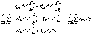 The Chebyshev expansions of terms
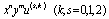 can be express as
 | (4) |
 | (5) |
 is a matrix of size
  and
and 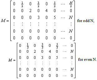 | (6) |
 are given in [10].Substituting the expressions (4), (5) and (6) into Eq. (1) and by simplifying the result , the following equation can be obtained.
 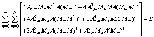 This equation can be written as
  | (7) |
 Matrix equation (7) can be transformed into a new matrix representation by using:
  Hence the following equation can be obtained.
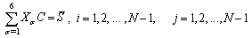 whereThus, the matrix equation can be obtained as
  Matrix representation of boundary conditions can be obtained by using the following relations:Similar to regulation of matrix equation (7), above boundary conditions can be transformed to the matrix equation
  whereand W is a matrix which is constructed by
  ,
,  ,
,  ,
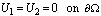
,  where I identity matrix.Consequently, using algebraic equation system obtained from differential equation and matrix representation of boundary conditions, we can get the main algebraic equation system. This system is solved to obtain the solution of the coefficients of the Chebyshev series.
 3. Application to Magnetohydrodynamic Flow Problem
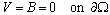
- Basic equations of fluid mechanics and Maxwell equations of electromagnetism are well known as coupled system of equations for velocity and magnetic field. In a rectangular duct
 , for the equations of steady, laminar, fully developed flow of viscous, incompressible and electrically conducting fluid are subjected to a constant and uniform applied magnetic field and they can be put in non- dimensional form[23]
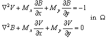 | (8) |
 | (9) |
 and
and  in Eq. (8) are velocity and induced magnetic field, respectively and the boundaries of the duct are assumed to be insulating. Hartmann number M is the norm of the vector
  The fluid is driven down the duct by means of a constant pressure gradient and
  ,
,  are parallel to z axis which is the axis of the duct. When the applied magnetic field intensity
  acts in a direction lying in the xy plane but forming an angle a with the y-axis, the following can be obtained:
 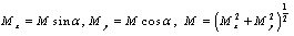 With the two new variables
 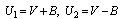 , Eq. (8) can be transformed into the following set of equations:
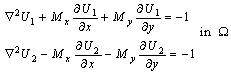 | (10) |
 . Hence, if
  is solved as
  from Eq. (10), then
  can be obtained directly. Thus by substituting
  , solution of original Eq. (8) can be obtained.If
  , then Eq. (10) can be written as
  with the boundary conditions
  .Approximate solution of the first differential equation of Eq.(10) is expressed in the truncated Chebyshev series as:
 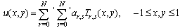 This solution can be expressed in the matrix form asPartial derivatives of the
  can be obtained as
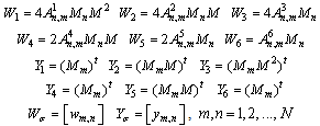
 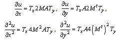 By substituting these equations in the first equation above and showing Hartmann number as “m” to not confuse with matrix M, the following can be obtained:Similar to regulation of Eq. (7), this equation can be regulated as where
  ,
,  Matrix representation of boundary conditions can be obtained by using the following relations:Similar to regulation of matrix equation (7), above boundary conditions can be transformed to the matrix equation
  .Hence, using algebraic equation system obtained from differential equation and matrix representation of boundary conditions, we have the main algebraic equation system which has
  unknowns whose rank is
  . From the solution of this system, we can find the coefficients of the Chebyshev series and the solution function as a Chebyshev series.
4. Numerical Results
- The Chebyshev collocation method is applied to solve the equation for
 with the boundary conditions
  . Solution
  can be obtained from solution
  as
as  which also satisfies
  .To solve the above equation, approximate solution has been taken as:
  Matlab is used to obtain the solution of resulting algebraic linear system of equations, constructed by applying the Chebyshev polynomial method. For several values of N and Hartmann numbers M up to 1000, and for the case that the applied magnetic field is parallel to the x axis
  , the solutions were obtained. For several values of N and Hartmann numbers M up to 700, the solution was carried out for directions of applied magnetic field such as
  and
and  . Solutions of the Chebyshev polynomial method which are shown by solid line (—) were compared with Sherciliff’s [24] exact solutions for
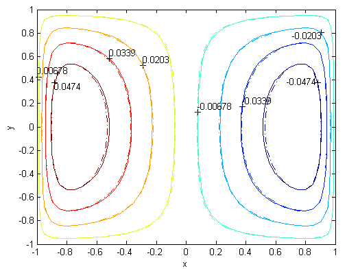
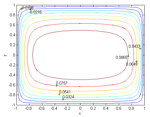
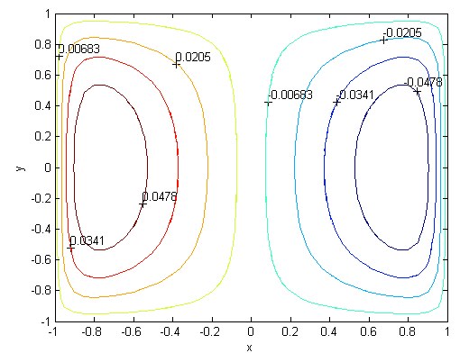
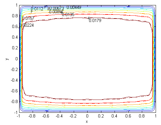
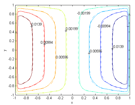
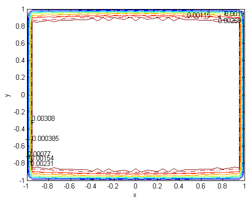
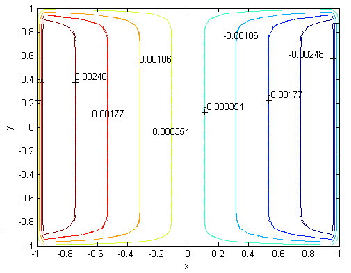
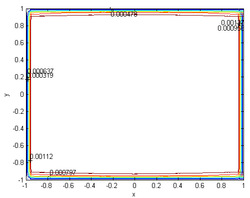
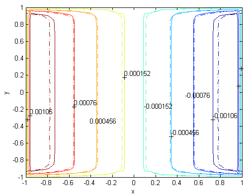
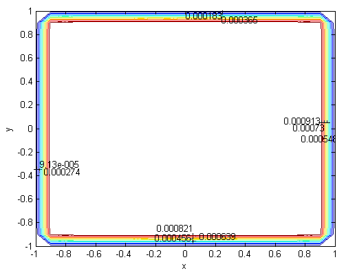
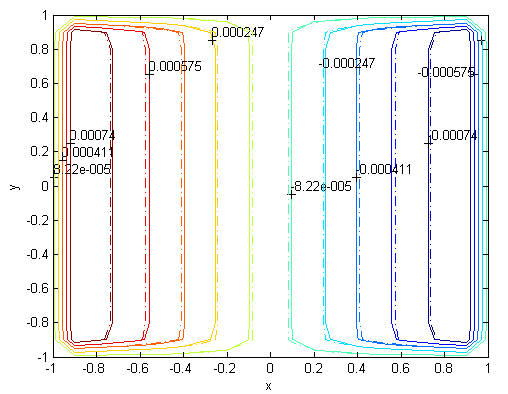
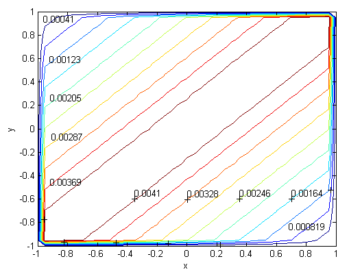
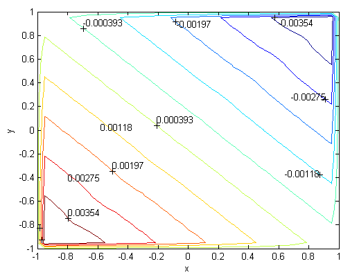
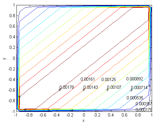
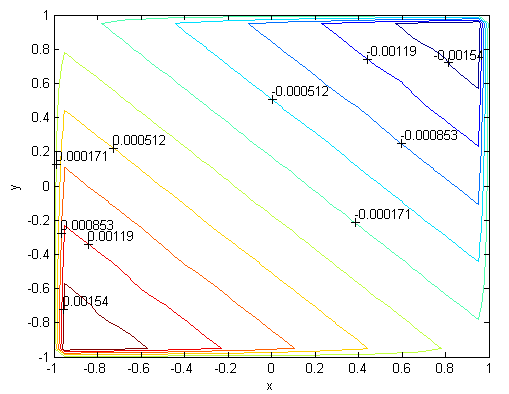
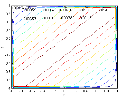
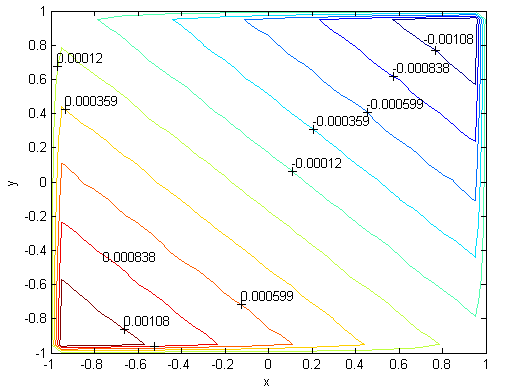
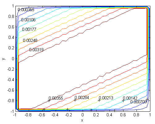
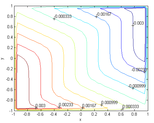
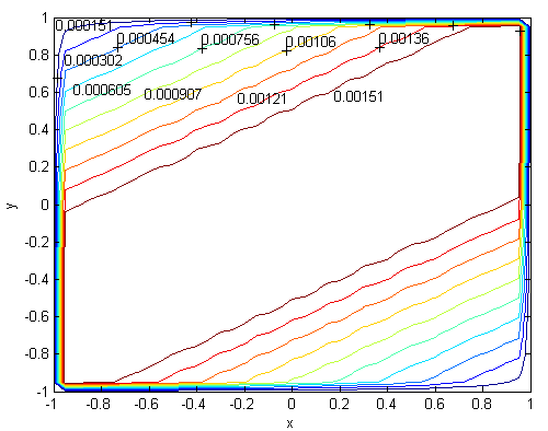
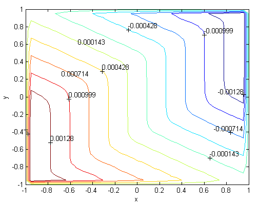
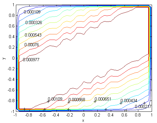
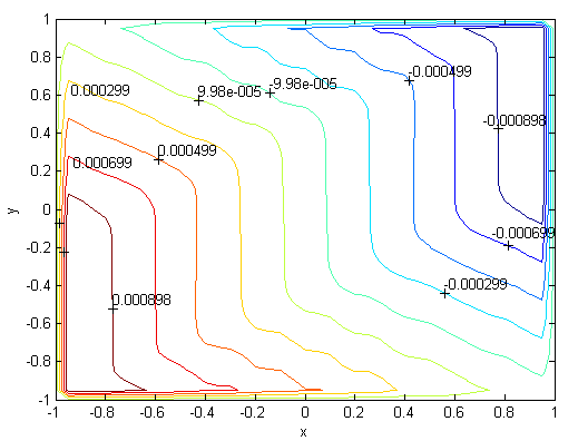
  which are shown by dash-dotted line (−∙−∙) in the figures.Figs. 1 and 2 represent the velocity and the induced magnetic field contours comparing the exact solution for Hartmann number M = 10 and N =11. Similarly, Figs. 3 and 4 show the results for M = 10 and N =13. Analyzing Figs 1and 3, Figs 2 and 4, it can be easily seen that computed values approach to the exact values when N is increased. The solution can be obtained for M = 50 with the value N =22 and results are given in Figs. 5 and 6 for the velocity and induced magnetic field contours. Figs. 7 and 8, Figs 9 and 10, Figs 11 and 12 represent the velocity and induced magnetic field contours for M =300, M =700, M =1000 respectively. It can be easily concluded that if the M is increased, the velocity and induced magnetic field become uniform at the center of the duct. In order to see the differences between computed values and exact solutions, lower values of N are used. If N is taken big enough, computed values and actual solutions overlap.Finally, Figs. 13 and 14, Figs. 15 and 16, Figs. 17 and 18, Figs. 19 and 20, Figs. 21 and 22, Figs. 23 and 24 present velocity and induced magnetic field contours with
  and
and  for M =300, M =700 and M =1000 respectively. This methodology can be used for the other value of
  . For the high Hartmann number, the boundary layer formation closer to the walls for both velocity and induced magnetic field is well observed. Velocity also becomes uniform at the center of the duct and flow becomes stagnant. The boundary layers are concentrated near the corners in the direction of the applied oblique magnetic field for both the velocity and induced magnetic field. These are the well-known characteristics of magnetohydrodynamic flow and are in agreement with our results.
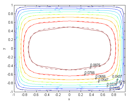 | Figure 1. Velocity, M=10, N=11,  |
 | Figure 2. Magnetic field, M=10, N=11,  |
 | Figure 3. Velocity, M=10, N=13,  |
 | Figure 4. Magnetic field, M=10, N=13,  |
 | Figure 5. Velocity, M=50, N=22,  |
 | Figure 6. Magnetic field, M=50, N=22,  |
 | Figure 7. Velocity, M=300, N=53,  |
 | Figure 8. Magnetic field, M=300, N=53,  |
 | Figure 9. Velocity, M=700, N=85,  |
 | Figure 10. Magnetic field, M=700, N=85,  |
 | Figure 11. Velocity, M=1000, N=99,  |
 | Figure 12. Magnetic field, M=1000, N=99,  |
 | Figure 13. Velocity, M=300, N=53,  |
 | Figure 14. Magnetic field, M=300, N=53  |
 | Figure 15. Velocity, M=700, N=85,  |
 | Figure 16. Magnetic field, M=700, N=85  |
 | Figure 17. Velocity, M=1000, N=93,  |
 | Figure 18. Magnetic field, M=1000, N=93  |
 | Figure 19. Velocity, M=300, N=53,  |
 | Figure 20. Magnetic field, M=300, N=53,  |
 | Figure 21. Velocity, M=700, N=85,  |
 | Figure 22. Magnetic field, M=700, N=85,  |
 | Figure 23. Velocity, M=1000, N=93,  |
 | Figure 24. Magnetic field, M=1000, N=93,  |
5. Conclusions
- This is the first time that MHD flow equation has been solved in a rectangular duct by using the Chebyshev polynomial method. This method has the capability of producing highly accurate solutions using considerably small numbers for N and it is an efficient method for larges values of Hartmann numbers M
 1000. From the figures, accuracy and efficiency of the method were demonstrated. Most commonly, in the previous studies, because of computational efforts, some difficulties were encountered for higher values of Hartmann numbers. In the Chebyshev polynomial method, considerably small number of N can be used so computational effort is less then others.