Nabil T. M. El-Dabe , M. H. M. Moussa , Rehab M. El –Shiekh , H. A. Hamdy
Department of Mathematics, Faculty of Education, Ain Shams UniversityHeliopolis, Cairo, Egypt
Correspondence to: Rehab M. El –Shiekh , Department of Mathematics, Faculty of Education, Ain Shams UniversityHeliopolis, Cairo, Egypt.
| Email: |  |
Copyright © 2012 Scientific & Academic Publishing. All Rights Reserved.
Abstract
In this paper, we use two integral methods, the first integral method and the direct integral method to study (2+1)- dimensional Davey-Stewartson equation . The first integral method was used to construct travelling wave solutions, those solutions are expressed by the hyperbolic functions, the trigonometric functions and the rational functions. By using the direct integration method shock wave solution and Jacobi elliptic function solutions are obtained. By comparison between the two methods, the direct integration is more impressive than the first integral method. The results obtained confirm that the proposed methods are efficient techniques for analytic treatment of a wide variety of nonlinear systems of partial differential equations.
Keywords:
(2+1)- Dimensional Davey-Stewartson Equation, The First Integral Method, The Direct Integral Method, Solitary Wave Solutions
1. Introduction
We consider the (2+1)-dimensional Davey-Stewartson equation[1].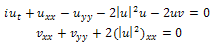 | (1) |
This equation is completely integrable and often used to describe the long time evolution of a two-dimensional wave packet[2,3]. In recent years, various methods such as inverse scattering, Darboux transformation, variable separation and Bäckland transformation have been used to solve the equation respectively[4-7]. The objectives of this work are twofold. First, we apply the first integral method[8-11] on the (2+1)-dimensional Davey-Stewartson equation to obtain solitary and periodic wave solutions. Second, we aim using the direct integration on the reduced nonlinear ordinary differential equation obtained after using the travelling wave transformation on the equation to get more exact solutions in the form of shock wave and Jacobi elliptic functions.
2. The First Integral Method
Consider the nonlinear partial differential equation in the from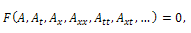 | (2) |
where A=A(x,t) is a solution of the nonlinear partial differential equation (2). We use the transformation | (3) |
where  This enables us to use the folowing changes:
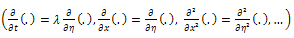 | (4) |
Using Eq. (4) to transfer the nonlinear partial differential Eq. (2) to nonlinear ordinary differential equation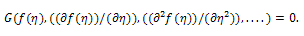 | (5) |
Next, we introduce a new independent variable | (6) |
which leads to a system of nonlinear ordinary differential equations | (7) |
By the qualitative theory of ordinary differential equations[12], if we can find the integrals to Eqs. (7) under the same conditions, then the general solutions to Eqs. (7) can be solved directly. However, in general, it is really difficult for us to realize this even for one first integral, because for a given plane autonomous system, there is no systematic theory that can tell us how to find its first integrals, nor is there logical way for telling us what these first integrals are. We will apply the Division Theorem to obtain one first integral to Eqs. (7) which reduces Eq. (5) to a first order integrable ordinary differential equation. An exact solution to Eq. (2) is then obtained by solving this equation. For convenience, first let us recall the division theorem for two variables in the complex domain C.Division Theorem : (see[13, 14]) Suppose that P(ω,z) and Q(ω,z) are polynomials in C[ω,z]; and P(ω,z) is irreducible in C[ω,z]. If Q(ω,z) vanishes at all zero points of P(ω,z), then there exists a polynomial G(ω,z) in C[ω,z] such that  | (8) |
3. The Application of the First Integral Method on the (2+1)-dimensional Davey-Stewartson Equation
In this section, we study the (2+1)-dimensional Davey-Stewartson equation using the first integral methodUse the transformation | (9) |
where k,  and
and  are constants, all of them are to be determined.Substituting Eq. (9) into Eq. (1), yield
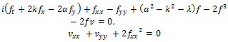 | (10) |
Using the transformation | (11) |
where  is a constant, system (11) become the following
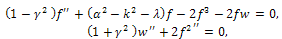 | (12) |
where prime denotes the differential with respect to  Integrating the second segment of Eq. (12) with respect to
  and taking the integration constant as zero yields
 | (13) |
Substituting Eq. (13) into the first segment of Eq. (12) we get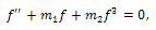 | (14) |
where 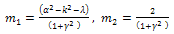 | (15) |
Using (7) we get | (16) |
 | (17) |
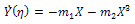
According to the first integral method, we suppose that  are nontrivial solutions of (16), (17) and
 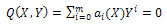 | (18) |
is an irreducible polynomial in the complex domain C[X,Y] such that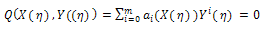 | (19) |
where (i=0,1,.......,m), are polynomials of X and
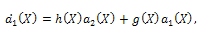
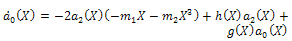
  Eq. (18) is called the first integral to (16), (17). Due to the Division Theorem, there exists a polynomial h(X)+g(X)Y, in the complex domain C[X,Y] such that
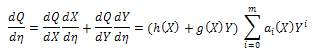 | (20) |
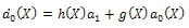
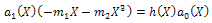
In this example, we take two different cases, assuming that m=1 and m=2 in (19), we haveCase 1:Suppose that m=1, by comparing with the coefficients of  on both sides of (20), we have
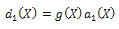 | (21) |
 | (22) |
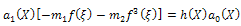 | (23) |
Since  (i=0,1) are polynomials, then from (21) we deduce that
  is constant and g(X)=0. For simplicity, take
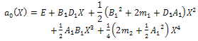
  =1, Balancing the degrees of h(X) and a₀(X), we conclude that deg(h(X))=1 only. Suppose that h(X)=AX+B, then from (22) we find a₀(X).
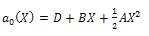 | (24) |
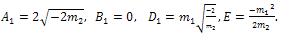
where A,B are arbitrary constants , and D is an arbitrary integration constant to be determined.Substituting a₀(X) and h(X) into (23) and setting all coefficients of X powers to be zero, then we obtain a system of nonlinear algebraic equations and by solving it, we obtain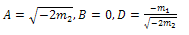 | (25) |
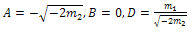 | (26) |
Using conditions (25) and (26) in Eq. (19), we obtain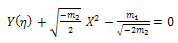 | (27) |
and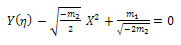 | (28) |
respectively. Combining Eq. (27) and Eq. (28) with Eq. (16), we obtain the exact solution to Eq. (16) and Eq. (17) and the exact solutions to the (2+1)-dimensional Davey- Stewartson equation can be written as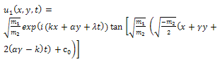 | (29) |
 | (30) |
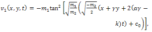
and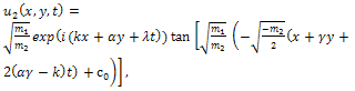 | (31) |
 | (32) |
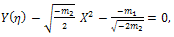
where  is an arbitrary integration constant,
  and
and  expressed by Eq. (15).Case 2Suppose that m=2, by comparing the coefficients of
 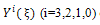 on both sides of (20),we have
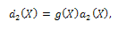 | (33) |
 | (34) |
 | (35) |
 | (36) |
Since  are polynomials, then from (33) we deduce that
  is a constant and g(X)=0, For simplicity, take
  , Balancing the degrees of h(X),
  we conclude that deg(h(X))=1 only. Suppose that
  , then from (34) and (35) we find
 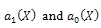 as follows
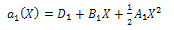 | (37) |
 | (38) |
where  are arbitrary constants, and
  are arbitrary integration constants.Substituting
  and h(X) in the last equation in (36) and setting all coefficients of X powers to be zero, then we obtain a system of nonlinear algebraic equations and by solving it with aid of Maple program, we obtain
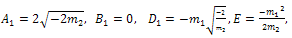 | (39) |
 | (40) |
Using conditions (39) and (40) into Eq. (19), we get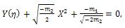 | (41) |
 | (42) |
Combining Eq. (41) and Eq. (42) with (16), we obtain the exact solution to Eq. (16)and Eq. (17) and the exact solution to Eq. (1) can be written as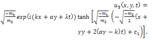 | (43) |
 | (44) |
and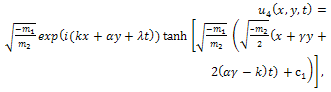 | (45) |
 | (46) |
where c1 is an arbitrary integration constant.
4. The Direct Method
In this section, we multiply Eq. (14) by  , then we get
 | (47) |
Case 1Integrating (47) once and considering the constant of integration to be zero, then we obtain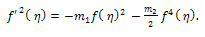 | (48) |
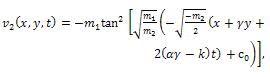
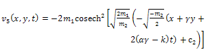
Eq. (44) has the following exact solution by using direct integration method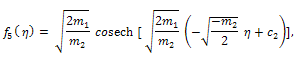 | (49) |
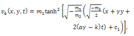
where c2 is an arbitrary integration constant.By back substitution we obtain the following new exact solution to the (2+1)-dimensional Davey- Stewartson equation 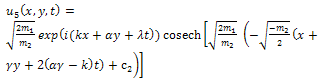 | (50) |
 | (51) |
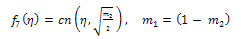
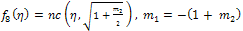
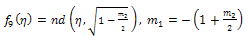
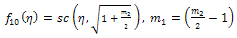
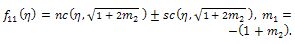
Case 2Integrating (43) once then we obtain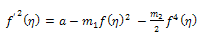 | (52) |
where a is an arbitrary integration constant.Using Jacobi functions, this equation have many solutions by relations between values of  and corresponding
  see[15], are given by the following
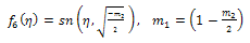 | (53) |
 | (54) |
 | (55) |
 | (56) |
 | (57) |
 | (58) |
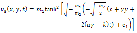
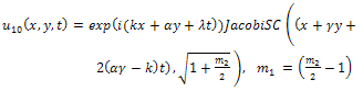
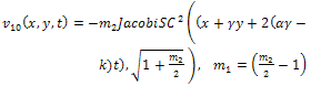
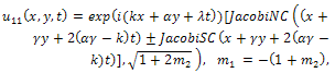
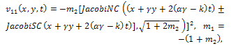
By back substitution we obtain the following new exact solutions of Eq. (1)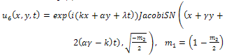 | (59) |
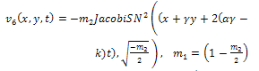 | (60) |
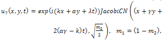 | (61) |
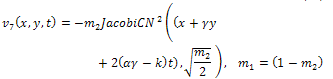 | (62) |
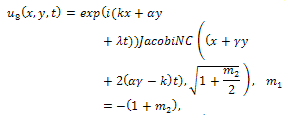 | (63) |
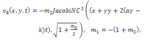 | (64) |
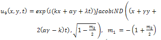 | (65) |
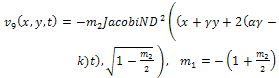 | (66) |
 | (67) |
 | (68) |
 | (69) |
 | (70) |
where  expressed by Eq. (15).All previous solutions are new and different from solutions mentioned in[1].
5. Conclusions
In this work, we have obtained many exact solutions of the (2+1 )-dimensional Davey-Stewartson equation by using the first integral method and the direct method. The application of the two methods was successfully used to establish travelling wave solutions for Eqs. (1). The two methods used have more advantages: it is direct and concise. By comparison between the two methods, the direct integral is more impressive than the first integral method.
References
| [1] | Zhao H., Chaos Solitons Fract. 36 (2008) 1283–1294. |
| [2] | Davey A., Stewartson K., Proc R Sco London ser A. 338 (1974) 101-110. |
| [3] | Tajirim M., Takeuchi K., Arai T. Phys Rev E. 64 (2001) 056622. |
| [4] | Ablowitz M. J., Segur H., Philadelphia PA:SIAM; (1981) 1-84. |
| [5] | Gu C. H., Hu H. S., Zhou Z. X., Shanghai Sci. Tech. publishing (1999) 79-97. |
| [6] | Lou S. Y., Lu J., J Phys A. 29 (1996) 4209-4215. |
| [7] | Paul S.K., Chowdhury A. R., J Nonlinear Math Phys. 5 (1998) 349-382. |
| [8] | Tascan F., Bekir A., Koparan M., Commun Nonlinear Sci Numer Simulat 14(2009)1810-1815. |
| [9] | Lu B., Zhang H. Q., Xie F. D., Appl. Math. Comput. 216 (2010) 1329-1336. |
| [10] | TaghiZadeh N., Milzazadeh M., Farahrooz F., Appl. Math. Model. 35(2011)3991-3997. |
| [11] | Hosseini R., Ansari R., Gholamin P., J. Math. Anal. 387(2012)807-814. |
| [12] | Ding T. R., Li C. Z., Peking University Press, Peking, 1996. |
| [13] | Feng Z., Chaos Solitons Fract. 38 (2008) 481-488. |
| [14] | Zhang T. S., Physics Letters A 371 (2007) 65-71. |
| [15] | Yomba E., Chaos Solitons Fract. 27 (2006) 187-196. |
 Abstract
 Reference
 Full-Text PDF
 Full-Text HTML