K. V. Zhukovsky
Faculty of Physics, Moscow State University, Leninskie Gory, Moscow, 119899, Russia
Correspondence to: K. V. Zhukovsky, Faculty of Physics, Moscow State University, Leninskie Gory, Moscow, 119899, Russia.
| Email: |  |
Copyright © 2012 Scientific & Academic Publishing. All Rights Reserved.
Abstract
We present a general method of operational nature to obtain solutions for several types of differential equations. Methodology of inverse differential operators for the solution of differential equations is developed. We apply operational approach to construct inverse differential operators and develop operational identities, involving inverse derivatives and generalized families of orthogonal polynomials. We employ them together with the exponential operator to investigate various differential equations. Advantages of operational technique for finding solutions of a wide spectrum of differential equations are demonstrated, in particular with regard to fractional differential equations.
Keywords:
Operator, Inverse, Differential Equation, Hermite, Laguerre Polynomials, Solution
Cite this paper: K. V. Zhukovsky, Inverse Derivative and Solutions of Some Ordinary Differential Equations, Applied Mathematics, Vol. 2 No. 2, 2012, pp. 34-39. doi: 10.5923/j.am.20120202.07.
1. Introduction
Understanding of differential equations and finding their solutions is of primary importance as for pure mathematics as for physics. With rapidly developing computer methods for the solutions of equations, the question of understanding of the obtained solutions and their application to real physical situations remains opened for analytical study. There are few types of differential equations, allowing explicit and straightforward analytical solutions. Indeed, expansion in series of orthogonal polynomials[1] is useful for solving many physical problems (see, for example, [2,3]). Such polynomials as Hermite, Laguerre and others are usually defined by series or sums. However, for the purpose of differential equations solution and in the context of operational approach to it, operational relations best define them. These polynomials possess generalized forms, including those with many variables and indices[4,7]. In what follows, we develop analytical method to obtain solutions for various types of differential equations on the base of operational identities, employing expansions in series of Hermite, Laguerre polynomials and their modified forms[1,5]. The key for constructing these solutions is operational approach and development of the formalism of inverse functions and inverse differential operators. We will demonstrate in what follows, that when properly used and combined, in particular, with integral transforms, such approach leads to elegant analytical solutions with transparent physical meaning without particularly cumbersome calculations.There are both practical and theoretical reasons for examining the process of inverting differential operators. Indeed, the inverse or integral form of a differential equation displays explicitly the input-output relationship of the system. Moreover, integral operators are computationally and theoretically less troublesome than differential operators; for example, differentiation emphasizes data errors, whereas integration averages them. Consequently, from theoretical point of view, it may be advantageous to apply computational procedures to differential systems, based on the inverse or integral description of the system. In mathematics, an inverse function is a function that undoes another function: If an input x into the function ƒ produces an output y, then putting y into the inverse function g produces the output x, and vice versa. i.e.,  and
and  or
or . If a function ƒ has an inverse ƒ −1, it is called invertible and the inverse function is then uniquely determined by ƒ. A relation can be determined to have an inverse if it is a one-to-one function. We can develop similar approach with regard to differential operators. The notation commonly used for the study of differential equations is designed rather for treating boundary conditions than for understanding of differential operators. Consequently, the concept of the inverse of a differential operator is not common. In what follows we will develop it and make use of operational technique to solve a variety of differential equations and produce useful relations, involving differential operators, special functions and series of extended forms of polynomials.
2. Inverse Derivative Technique
Let us denote a common differential operator  . The inverse derivative of a function ƒ(x) is another function F(x):
 | (1) |
whose derivative is . Naturally, we expect anti-derivative or inverse derivative
  as the inverse operation of differentiation to be an integral operator. The generalized form of the inverse derivative of ƒ(x) with respect to x evidently is
 , where C — the constant of integration. The action of the inverse derivative operator of the n-th order
 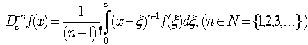 | (2) |
can be complemented with the definition for its zeros order action as follows: | (3) |
Hence, we can write: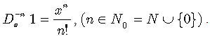 | (4) |
Consider a general form of differential equation  | (5) |
where  — differential operator composed of derivatives or various orders: D, D2,…, Dn. We can define the inverse differential operator
  or
or , such that
  | (6) |
From (5) we obtain  | (7) |
and, since it satisfies (5), the particular integral of (5) is given by . The inverse differential operator
  is linear, i.e.
  | (8) |
where a and b — constants, ƒ(x) and g(x) — some functions of x. To illustrate usefulness of the concept of inverse differential operator, let us consider the following operator :
: | (9) |
where c0 and c1 — constants. Consider the following equation: 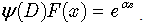 | (10) |
The action of  on exp(αx) results in
  | (11) |
Now, applying inverse operator  to both sides, we obtain:
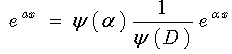 | (12) |
or  | (13) |
The above formula yields the conclusion, that eq.(10) possesses the following particular integral: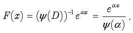 | (14) |
Following the above steps, it can be easily shown by means of inverse derivative operator, that (14), being the solution of eq.(10), is true also for the operator  with higher than second order derivatives. Moreover, the inverse derivative operator makes it is easy to prove the following identity:
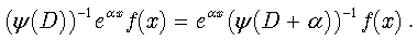 | (15) |
Indeed, differentiation of the 1st and 2d order of  yields
 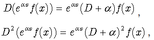 | (16) |
and so on. Thus, we write: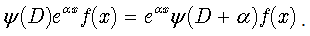 | (17) |
Now we adopt the notations 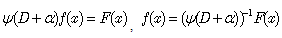 | (18) |
and we obtain from (17) the following equality: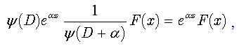 | (19) |
which, upon the action of the inverse derivative (ψ(D))-1 on both sides, gives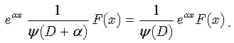 | (20) |
By replacing F(x) ↔ ƒ in eq.(20), it becomes evident that the action of the inverse operator  on a function ƒ can be expressed via the inverse differential operator
  as follows:
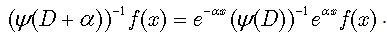 | (21) |
Derivative operator D in the l.h.s. is the simplest example of . We formally solve the differential equation
  as follows:
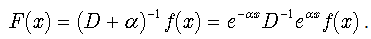 | (22) |
For  we evidently have
  . Obviously, for
  we obtain the solution of the equation
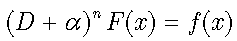 | (23) |
in the following form: | (24) |
where the action of  can be calculated according to (2). For example, if
  in the r.h.s., then we immediately obtain
  . Let us consider the following general form of this equation:
  | (25) |
where we denote operator  and α, β — constants. In order to find the particular integral
 | (26) |
we shall make use of the well-known operational identity [5,6]: | (27) |
which reads for the operator :
: | (28) |
The differential operator  in the exponential reduces to the first order derivative with the help of the following integral presentation for the exponential of a square of an operator
 :
: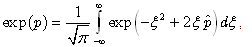 | (29) |
where  in our case. Thus, the above formula reads as follows:
 | (30) |
Now, if we take into account the action of the operator of translation  for
for :
: | (31) |
the above-sketched operational procedure yields the following expression for the particular integral (26):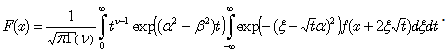 | (32) |
Upon performing the change of variables, given by 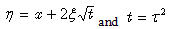 | (33) |
we finally obtain: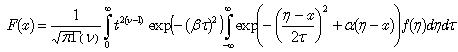 | (34) |
Assuming ν = 1, we evidently obtain a simpler expression:  | (35) |
When α = β in (25) further simplification follows: 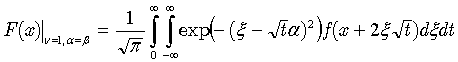 | (36) |
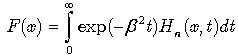
If α = 0 in eq.(25), then for the equation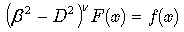 | (37) |
we write the following solution: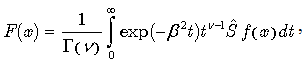 | (38) |
where the differential operator 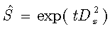 | (39) |
was explored by Srivastava in[6]. In particular, if  , we can employ the generalized form of the Glaisher operational rule[6]
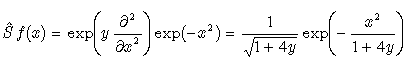 | (40) |
to obtain the particular solution as follows: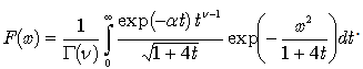 | (41) |
So far, we have demonstrated on simple examples how the usage of the inverse derivative together with operational formalism, in particular, with the exponential operator technique, provide elegant and easy way to find solutions in some classes of differential equations. In what follows we will apply the concept of inverse derivative to find solutions of more sophisticated problems, expressed by differential equations.
3. Inverse Differential Operators and Orthogonal Polynomials
Let us consider some polynomials and their generalised forms from operational point of view, rather than their traditional expansions in series. We will explore the relations between exponential operator of derivatives and inverse derivatives on one side, polynomials and special functions on the other side. Recently, Srivastava, Dattoli and Zhukovsky reconsidered Hermite, Laguerre and other polynomial families by means of operational technique[4,7] and[8]. Hermite polynomials of two variables are explicitly given by following operational rule[4] and by the series expansion [9]: 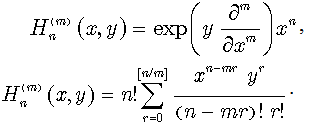 | (42) |
Note, that  | (43) |
where  are more commonly known Hermite polynomials of two variables
 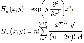 | (44) |
with the following generating function: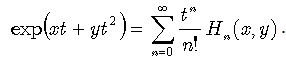 | (45) |
They can be reduced to the well-known forms of Hermite polynomials of single variable: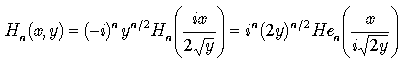 | (46) |
Hermite polynomials also satisfy the following useful and easy to prove relation  | (47) |
Laguerre polynomials of two variables can be given by an operational relation[4] or a sum as follows: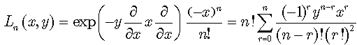 | (48) |
They also reduce to polynomials of a single variable[6] as follows: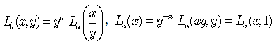 | (49) |
There is a definite meaning in the introduction of the second variable in Hermite and Laguerre polynomials. It essentially allows us to consider them as solutions of partial differential equations with proper initial conditions: 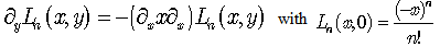 | (50) |
for Laguerre polynomials  and
and  | (51) |
for Hermite polynomials  . Note that the following differential operators
 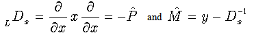 | (52) |
are non commutative: 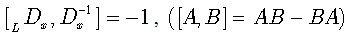 | (53) |
and the following operational relation between them exists [8]: 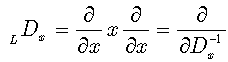 | (54) |
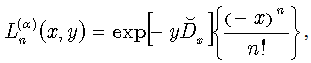
With the help of this relation, we can extend our approach on differential equations, including operator  , sometimes called Laguerre derivative
  . Then, from the definition (52) we immediately conclude for Laguerre polynomials
  , defined in (48), that in terms of inverse derivative operator they are expressed as follows:
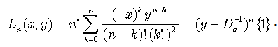 | (55) |
Moreover, it follows from (48) and (55) that the following operational identity is true for Laguerre polynomials: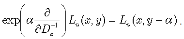 | (56) |
Extensive study of the relations between various polynomial families, inverse derivative operator, exponential operator and realization of operators  and
and , which stand respectively for multiplicative operator and differential operator for quasi-monomial polynomials, can be found in [14] and [15]. Various polynomial families, such as Hermite, Laguerre, Legendre, Shaffer and hybrid polynomials were discussed there in the context of a more general family of Appèl polynomials, which they belong to. Such consideration became possible in the framework of operational approach, where inverse derivative plays important role as an instrument for the study of relevant polynomial families, their features and properties. In what follows, we will mainly focus on the technique of inverse operator, applied for derivatives of various orders and their combinations. We will demonstrate that, when combined with integral transforms and operational relations for various polynomial families, it allows for easy and straightforward solutions of various types of differential equations. First, note that if we choose the function
  in the r.h.s. of (25) with α = 0, then, upon the action of the exponential operator, we obtain from (28) the two-variable Hermite polynomials (44) in the integral:
 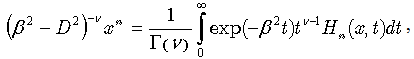 | (57) |
and the particular solution for (25) in the simplest case of ν = 1, α = 0,  :
:  | (58) |
Even without specifying the values of ν and α and the type of the function f in the r.h.s. of (25), we can still disentangle two integrals in (34) by involving Hermite polynomials of two variables (45) as follows: 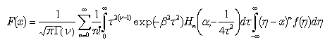 | (59) |
Consider, for example, the following equation:  | (60) |
From operational point of view, its solution evidently writes as follows: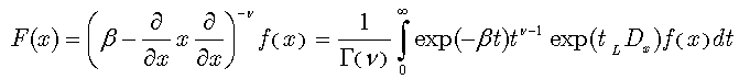 | (61) |
Note, that the above formula is valid for any fractional ν and thus we have effectively obtained (61) solution of a fractional differential equation (60). For  this integral presentation reduces to Laplace transforms for the differential operator
  , involved in (61), identical, except for the change
  , to the well known Laplace transforms for the operator
  , written below:
 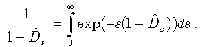 | (62) |
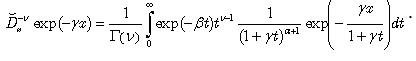
The choice of the initial condition function  in (61) yields the following identity:
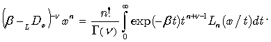 | (63) |
Moreover, we can either write a solution of for an arbitrary function , if only its expansion into series of simple Laguerre polynomials
  exists. Then, provided
 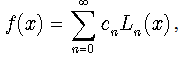 | (64) |
and taking into account (56), the solution (61) of equation (60) can be also written as the following integral of series of Laguerre polynomials: 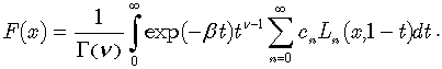 | (65) |
For the exponential function  we can make use of the generalized form of the Glaisher operational rule[10]
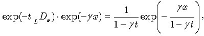 | (66) |
which immediately produces the following result: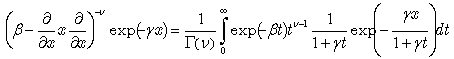 | (67) |
Again, we underline that this result is valid for fractional ν and thus allows the solution of a fractional differential equation. Another interesting case arises when we consider the equation similar to (25) with Laguerre derivative  instead. Let us choose the following initial condition function:
  | (68) |
where 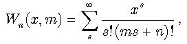 | (69) |
 — a particular case of the Bessel-Write function[6]. Then, following (27), we can write the solution:
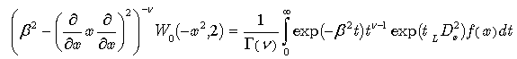 | (70) |
Eventually, based on the operational definition of Laguerre polynomials (48) and exploiting another generalized form of Glaisher operational rule[8] in the form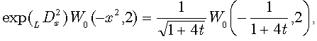 | (71) |
we obtain: 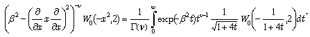 | (72) |
Moreover, according to the developed above procedure, we can write solutions for other than specified above types of equations. For example, we can take advantage of the generalization of Laguerre polynomials  :
: | (73) |
where operator  is defined as follows:
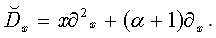 | (74) |
Inverse operator technique easily allows us to write the solution of the equation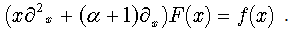 | (75) |
Indeed, by following operational rule (27), we get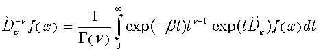 | (76) |
and for initial condition function  , previously met in the context of eq.(25), we now write:
 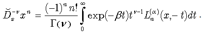 | (77) |
Similarly to (63), taking advantage of the generalized form of the Glaisher operational rule from [6], we obtain for the operator  and
and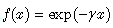 :
: | (78) |
4. Conclusions
Operational methods provide fast and universal mathematical tool for obtaining solutions of differential equations. Combining operational methods, integral transforms and the theory of special functions and orthogonal polynomials, we get even more powerful analytical instrument for solving a wide spectrum of differential equations and relevant to them physical problems. Generalized orthogonal polynomials, in particular, of Laguerre and Hermite families, provide a possibility to write solutions in most general cases in form of series or sums and allow for compact form of the solutions, facilitating their analysis. Moreover, they frequently give links to special functions, which is sometimes even more advantageous. In conclusion, we would like to underline that in the present article we demonstrated how the technique of inverse operator, applied for derivatives of various orders and their combinations, combined with integral transforms, allows for easy and straightforward solutions of various types of differential equations. By means of operational method, we developed the methodology of inverse differential operators and derived a number of operational identities, involving various inverse differential operators. We have demonstrated that, using the technique of inverse derivatives and inverse differential operators, we can make significant progress in treatise of a variety of mathematical problems, related to solutions of differential equations. In the following paper, we will investigate the possibilities, which operational approach opens, to solve partial differential equations. We will use inverse derivatives and inverse differential operator’s formalism, developed in our present work and combined with exponential operator, integral transforms and special functions.
References
| [1] | A. Appèl and J. Kampé de Fériet, Fonctions Hypergéométriques et Hypersphériques; Polynômes d’Hermite, Gauthier-Villars, Paris, 1926. |
| [2] | D. T. Haimo and C. Markett, A representation theory for solutions of a higher-order heat equation. I, J. Math. Anal. Appl. 168 (1992) 89. |
| [3] | D. T. Haimo and C. Markett, A representation theory for solutions of a higher-order heat equation. II, J. Math. Anal. Appl. 168 (1992) 289. |
| [4] | G. Dattoli, Generalized polynomials, operational identities and their applications, J. Comput. Appl. Math. 118 (2000) 111. |
| [5] | A. Erdélyi, W. Magnus, F. Oberhettinger and F. G. Tricomi, Higher Transcendental Functions, Vol. II, McGraw-Hill Book Company, New York, Toronto and London, 1953. |
| [6] | H. M. Srivastava and H. L. Manocha, A Treatise on Generating Functions, Halsted Press (Ellis Horwood Limited, Chichester), John Wiley and Sons, New York, Chichester, Brisbane and Toronto, 1984. |
| [7] | G. Dattoli, H. M. Srivastava and K. Zhukovsky, Оrthogonality properties of the hermite and related polynomials, J. Comput. Appl. Math. 182 (2005) 165. |
| [8] | G. Dattoli, H. M. Srivastava and K. Zhukovsky, A new family of integral transforms and their applications, Integral Transform. Spec. Funct. 17, N1 (2006) 31. |
| [9] | H.W. Gould, A.T. Hopper, Operational formulas connected with two generalizations of Hermite polynomials, Duke Math. J. 29 (1962) 51–63. |
| [10] | G. Dattoli, H. M. Srivastava, K. V. Zhukovsky, Operational methods and Differential Equations with Applications to Initial-Value problems, Appl. Math. Comput. 184 (2007) 979. |
| [11] | K. B. Wolf, Integral Transforms in Science and Engineering, New York Plenum Press, 1979. |
| [12] | G. N. Watson, A Treatise on the Theory of Bessel Functions, Second Edition, Cambridge University Press, Cambridge, London and New York, 1944. |
| [13] | J. E. Avron and I. W. Herbst, Spectral and scattering theory of Schrödinger operators, related to the stark effect, Commun.Math.Phys. 52 (1977) 239. |
| [14] | G. Dattoli, K.V.Zhukovsky, Appèl Polynomial Series Expansion, Int. Math. Forum 5, N14 (2010) 649. |
| [15] | G. Dattoli, M. Migliorati, K.Zhukovsky, Summation Formulae and Stirling Numbers, Int. Math. Forum 4, N41 (2009) 2017. |
 Abstract
 Reference
 Full-Text PDF
 Full-text HTML