R. Nageshwar Rao , P. Pramod Chakravarthy
Department of Mathematics, Visvesvaraya National Institute of Technology, Nagpur, 440010, India
Correspondence to: P. Pramod Chakravarthy , Department of Mathematics, Visvesvaraya National Institute of Technology, Nagpur, 440010, India.
| Email: |  |
Copyright © 2012 Scientific & Academic Publishing. All Rights Reserved.
Abstract
In this paper, we present a numerical patching technique for solving singularly perturbed nonlinear differential-difference equation with a small negative shift. The nonlinear problem is converted into a sequence of linear problems by quasilinearization process. After linearization, it is divided into two problems, namely inner region problem and outer region problem. The boundary condition at the cutting point is obtained from the theory of singular perturbations. Using stretching transformation, a modified inner region problem is constructed and is solved by using the upwind finite difference scheme. The outer region problem is solved by a Taylor polynomial approach. We combine the solutions of both problems to obtain an approximate solution of the original problem. The proposed method is iterative on the cutting point. The process is repeated for various choices of the cutting point, until the solution profiles stabilize. Some numerical examples have been solved to demonstrate the applicability of the method. The method is analyzed for stability and convergence.
Keywords:
Singular Perturbations, Numerical Patching Technique, Nonlinear Differential-Difference Equation, Upwind Finite Difference Scheme, Taylor Polynomial Approach
1. Introduction
A singularly perturbed differential-difference equation is an ordinary differential equation in which the highest derivative is multiplied by a small parameter and involving at least one delay term. Such problems are found throughout the literature on epidemics and population dynamics where these small shifts play an important role in the modeling of various real life phenomena[10]. Boundary value problems in differential difference equations arise in a very natural way in studying variational problems in control theory where the problem is complicated by the effect of time delays in signal transmission[12]. In the mathematical model for the determination of the expected first-exit time in the generation of action potential in nerve cells by random synaptic inputs in dendrites, the shifts are due to the jumps in the potential membrane which are very small[11]. In[5] the authors C.G. Lange and R.M. Miura gave an asymptotic approach in the study of a class of boundary value problems for linear second order differential-difference equations in which the highest order derivative is multiplied by a small parameter. In[4] the authors have extended the ideas to the boundary value problems for singularly perturbed nonlinear differential difference equations and discussed the existence and uniqueness of their solutions. In[3], the authors proposed a numerical method to solve the boundary value problems for singularly perturbed linear differential-difference equations, which worked well when the delay parameter is of O(ε) or o(ε). To handle the delay argument, they constructed a special type of mesh so that the term containing delay lies on nodal points after discretization. Mustafa Gulsu and Mehmet Sezer[6] have proposed a Taylor polynomial approach for solving mth order linear differential-difference equations with mixed conditions. This method is based on first taking the truncated Taylor’s expansions of the functions in the differential-difference equations and then substituting their matrix forms into the equation. Hence the result matrix equation can be solved and the unknown Taylor coefficients can be found approximately. In[1], the authors M.K. Kadalbajoo and K.K. Sharma presented the numerical study to solve the singularly perturbed nonlinear differential difference equations with negative shift. When the shift is o(ε), the term containing the shift is expanded in Taylor series and when the shift is O(ε), a special type of mesh is constructed to handle the shift term. In[2], the authors M.K.Kadalbajoo, Devendra Kumar proposed a B-Spline collocation method for solving a singularly perturbed nonlinear differential difference equation with negative shift. A piecewise uniform mesh is used to grasp the better approximation to the exact solution in the boundary layer region. Taylor series is used to tackle the delay.In this paper, we present a numerical patching technique for solving singularly perturbed nonlinear differential difference equations with negative shift and present the numerical study to such problems. In order to know the behaviour of the solution of the singularly perturbed differential difference equations in the boundary layer region, it is always suggestive to divide the original problem into two problems namely, the inner region problem and the outer region problem and solve them separately. First, we linearize the nonlinear boundary value problem using quasilinearization[8] and obtain a sequence of linear boundary value problems. Then it is divided into two problems namely inner region problem and outer region problem. The boundary condition at the cutting point is obtained from the theory of singular perturbations. Using stretching transformation, a modified inner region problem is constructed and is solved by using the upwind finite difference scheme. The outer region problem is solved by a Taylor polynomial approach given by Mustafa Gulsu and Mehmet Sezer[6]. We combine the solutions of both the problems to obtain an approximate solution to the original problem. The proposed method is iterative on the cutting point. The process is to be repeated for various choices of the cutting point, until the solution profiles stabilize. The existence and uniqueness of the discretized problem along with stability estimates are discussed. Some numerical examples have been solved to demonstrate the applicability of the method.
2. Numerical Patching Technique
To describe the method, we first consider a nonlinear singularly perturbed differential difference equation of the form: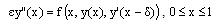 | (1) |
subject to the interval and boundary conditions  | (2) |
where  is a small perturbation parameter and
  . The solution y(x) of the boundary value problem (1)-(2) is assumed to be continuous on[0,1] and continuously differentiable on (0,1).It is assumed that
 is smooth function satisfying the conditions:
 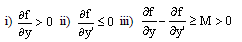 , where M is a positive constant.iv) The growth condition
  as
as  for all x∈[0,1] and all real y and
  .For δ=0, under the conditions listed above the problem (1)-(2) has a unique solution[9].To develop a numerical scheme for the boundary value problem (1)-(2), we first linearize the original nonlinear problem by using quasilinearization process[8]. The nonlinear differential equation is linearized around a nominal solution of the nonlinear differential equation which satisfies the specified boundary conditions. Let
  be the initial guess to the solution of the problem (1) satisfying the boundary conditions
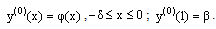 Then a sequence of boundary value problems can be obtained as follows:We have
  | (3) |
with , –δ≤x≤0;
  Expanding the right hand side of (3) in Taylor series about
  , we obtain
 | (4) |
By rearranging the terms of (4) we obtain the recurrence relation of singularly perturbed linear differential-difference equations  | (5) |
with  For simplicity, we denote
 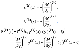 Then (5) may be written as
  | (6) |
with 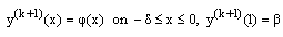 | (7) |
The solution of the reduced problem of (1)-(2) is assumed to be the initial approximation  , and the successive approximations
  are determined by (6)-(7). Hence, instead of solving the original nonlinear problem (1)-(2), we solve the sequence of boundary value problems for singularly perturbed second order linear differential equations with negative shift given by (6)-(7) for k=0,1,2, For large values of k the solutions
  converge to the solution
  of the original nonlinear differential equation while numerically, we require that
  ,
,  , where μ is the prescribed tolerance. The iteration can be terminated when the above condition is satisfied, and the profile
  is the numerical solution of the nonlinear boundary value problem (1)-(2). Due to the presence of the singular perturbation parameter
 , the solution of the problem exhibits boundary layer behavior. As ε→0, the order of the reduced problem decreases by one, therefore the solution exhibits boundary layer behavior at either of the boundary points i.e., the boundary layer will be on the left side or the right side of the domain of consideration depending on the sign of the coefficient
  of the convection term that is according as
  or
or  respectively, where M is a positive constant. We assume that
  throughout the interval [0, 1]. This assumption implies that the boundary layer will be in the neighborhood of x=0. We set δ=τε with τ=O(1). If τ is not too large, the layer structure is modified but maintained at the same end [5]. We consider
  the cutting point or the thickness of the boundary layer. Now the linearized problem is divided into two problems namely the inner region problem and the outer region problem. The inner region problem is defined in the interval
  and the outer region problem is defined in the interval
  .
.
2.1. Boundary Condition at the Cutting Point
We assume that  are sufficiently differentiable. By expanding the retarded term
  using Taylor series, we obtain
  Since δ=τε, we have
 | (8) |
By substituting (8) in (6), we get  | (9) |
We shall seek an outer solution as an asymptotic expansion in the form  | (10) |
where  are unknown functions to be determined. Substituting (10) in (9) and simplifying, we get
 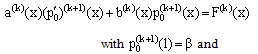 | (11) |
 | (12) |
The solution of (11) is  The functions
  can be obtained by solving equation (12) for n=1,2,3. Thus the expansion for
  given in equation (10) is obtained. Hence the boundary condition at the cutting point can be obtained from (10) and denote
 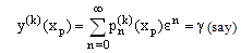 | (13) |
Since the terminal point  is common to both the inner and outer regions, it defines the inner region problem as a boundary value problem
 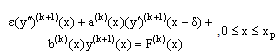 | (14) |
with the interval and boundary conditions  | (15) |
and the outer region problem as a boundary value problem 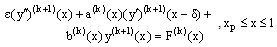 | (16) |
with the boundary conditions  | (17) |
2.2. Inner Region Problem
From (14)-(15) the inner region problem is given by 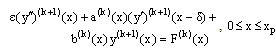 | (18) |
with the interval and boundary conditions  | (19) |
We choose the transformation x=tε to create a new inner region problem. By rescaling the equation (18) with 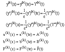 | (20) |
we obtain the new differential-difference equation for the inner region solution as  | (21) |
where  .The boundary conditions for the equation (21) are determined by (19) and (20) as
 | (22) |
We solve the new inner region problem (21)-(22) to obtain the solution over the interval . We construct a numerical scheme for solving (21)-(22) based on an upwind finite difference scheme. We divide the interval
  into n equal parts. To tackle the delay term, we choose the mesh parameter as
 , where m=pq, p is a positive integer and q is the mantissa of
  . The difference scheme for (21)-(22) is given by
  | (23) |
 | (24) |
and where
where  ,
, and
and  Now (23)-(24) become
 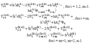 | (25) |
with 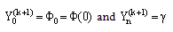 | (26) |
The discrete problem (25)-(26) reduces to a system of (n+1) linear difference equations given by  | (27) |
where  ,
,  and
and  , the nonzero entries of the system matrix being given by
  and
and 
 The system (27) is solved by Gauss elimination method with partial pivoting. In fact, any numerical method or analytical method can be used.
2.3. Outer Region Problem
Since the terminal point is common to both the inner and outer regions, it defines the outer region problem as a boundary value problem
 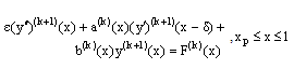 | (28) |
with the boundary conditions  | (29) |
We solve the outer region problem (28)-(29) by employing the Taylor polynomial approach given by Mustafa Gulsu and Mehmet Sezer[6] to obtain the solution over the interval .
.
2.4. Solution of the Original Problem
After getting the solution of the inner region problem and outer region problem, we combine both to obtain the approximate solution of the original problem (1)-(2) over the interval 0 ≤x≤ 1. We repeat the process for various choices of xp, until the solution profiles do not differ materially from iteration to iteration. For computational purposes we use an absolute error criterion, namely  where
where  is the ith iterate of the inner region solution and
  is the prescribed tolerance bound.
3. Error Estimate
Now we shall find the error estimate for the modified inner region problem (23) under the boundary conditions (24). Throughout the analysis simplicity we replace  with
with  respectively. Case 1: When
 , where θ is a positive constant. Lemma 1: (Discrete minimum principle)Let
  be any mesh function that satisfies
  and
and  and
and  then
then  for all i = 0,1,2,…, n. Proof: Let
  be such that
  and assume that
 .Clearly
  . Then for
  we have We have
 since
since  Thus, we have
  which contradicts the hypothesis that
  for
for  of the discrete minimum principle. This contradiction arose since we assumed that
 . Therefore our assumption is wrong. Hence,
  . But
. But  is an arbitrary positive integer, so
  for all
  .Theorem 1: If
  and
and , where M and θ are positive constants, then the solution of the discrete problem (23) with the boundary conditions (24) exists, is unique and satisfies
  | (30) |
where  is a positive constant. Here,
  is the discrete
  norm defined by
  Proof: Suppose
  and
and  be two solutions to the discrete problem (23), (24). Then,
  is a mesh function satisfying
  for
for , we have
  .Since
  and
and satisfy (25), therefore
 .Thus, the mesh function
  satisfies the hypothesis of the discrete minimum principle and so by the application of it to the mesh function
  we get
  | (31) |
Again let  , then
 satisfies
  and proceeding as above we get
  . Thus, the discrete minimum principle can be applied for the mesh function
  which gives
 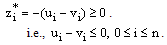 | (32) |
Hence, from (31) & (32) we get  , which prove the uniqueness of the solution to the discrete problem (23)-(24) and for linear equations, the existence is implied by uniqueness. Now to prove the bound on
  we consider two barrier functions
  defined by
 , 0≤i≤n where
  is an arbitrary positive constant. Then, we have
 , since
 and
and 
 , since
 since
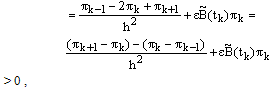
since  For
For  , we have
 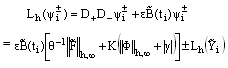 | (33) |
Also for  , we have
 Then from (33) we get
  Since,
  , that is
  , we get
  | (34) |
Since, in the above inequality (34) the first and second terms are negative, so we choose the constant K such that the sum of the moduli of the first and second terms dominates the modulus of the third term in the above inequality. We then obtain | (35) |
For  ,we have
 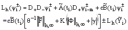 | (36) |
We know that for i=m, m+1,..,n-1,  Then from (36) we get
  Since,
  , that is
  , we get
 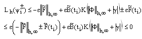 | (37) |
Hence,  (38)Combining the results of (35) and (38) we get
  .Thus an application of Lemma 1 to the mesh function
  gives
gives  which proves the required bound on the discrete solution
  .Case 2: When
  , where θ is a positive constant. Lemma 2: (Discrete maximum principle)Let
  be any mesh function that satisfies
  and
and  and
and  then
then  for all i=0,1,2,…,n.Proof: Let
  be such that
  and assume that
  .Clearly
  . Then, for
  we have
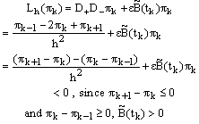 Thus, we have
  which contradicts the hypothesis that
  for i=1,2,…,n-1 of the discrete maximum principle. This contradiction arose since we assumed that
  . Therefore our assumption is wrong. Hence,
  . But
. But  is an arbitrary positive integer, so
  for all i=1,2,…,n.Theorem 2: If
 and
and  , where M and θ are positive constants, then the solution of the discrete problem (23) with the boundary conditions (24) exists, is unique and satisfies
  | (39) |
where  is a positive constant. Proof: Let
  and
and  be two solutions to the discrete problem (23), (24). Then,
  is a mesh function satisfying
 , we have
  Since
Since  and
and satisfy (23), therefore
  .Thus, the mesh function
  satisfies the hypothesis of the discrete maximum principle and so by the application of it to the mesh function
  we get
  | (40) |
Again we consider , then
  is a mesh function satisfying
  and proceeding as above we get
  . Thus, the discrete maximum principle is applied on the mesh function
  which gives
  | (41) |
Hence, from the (40), (41) we get  , for
, for  which proves the uniqueness of the solution to the discrete problem (23)-(24) , and for linear equations the existence is implied by uniqueness. Now to prove the bound on
  we consider two barrier functions
  defined by
  ,where
  is an arbitrary positive constant. Then, we have
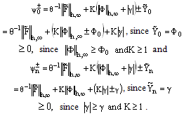 and for
  we have
 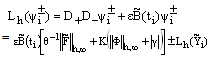 | (42) |
We know that for i=1,2,..m-1,  Then from (42) we get
  Since,
  , that is
  , we get
 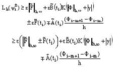 | (43) |
Since, in the above inequality (43) the first and second terms are positive, so we choose the constant K so that the sum of the moduli of the first and second terms dominates the modulus of the third term in the above inequality. We then obtain | (44) |
For  , we have
 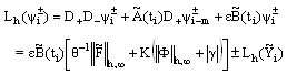 | (45) |
We know that for i=m, m+1,.., n-1,  Then from (45) we get
 Since,
  , that is
  , we get
 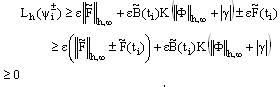 | (46) |
Hence,  (47)Combining the results of (44) and (47) we get
  .Thus an application of Lemma 2 to the mesh function
  gives
gives  which proves the required bound on the discrete solution
  .Thus, Theorems (1) and (2) imply that the solution to the discrete problem (23), (24) is uniformly bounded, independently of the mesh parameter h and the parameter
  , which proves that the difference scheme is stable for all mesh sizes. Corollary: Under the assumption that
 , the error
  between the solution
  of the continuous problem (21), (22) and the solution
  of the discrete problem (23),(24) satisfies the estimate
  , where
  satisfies
 Proof: The truncation error
  is given by
  Now using Taylor’s series and after simplifications, we obtain
  We have
 i=1,2,…,n-1 and e0=en= 0.Then by using Theorems (1) and (2) we obtain the required error estimate.
4. Numerical Results
We have applied the present method on two nonlinear singularly perturbed differential-difference equations with small negative shift. The nonlinear problems are first converted into sequence linear singularly perturbed differential-difference equations by using quasilinearization method. The solution of the reduced problem is taken as initial approximation. Example 1[2, p.2593]:  , with the interval and boundary conditions
  The solution at the cutting point is given by the reduced problem solution
  where
where and
and  and hence
  The linearized form of the given nonlinear equation by quasilinearization method is
  with the conditions
  and
and  .The modified inner region problem is given by
  , 0 ≤ t ≤ tp under the conditions
 ,
,  .The outer region problem is given by
  , xp≤x≤ 1 under the conditions
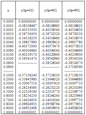
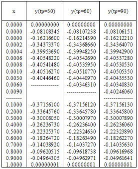
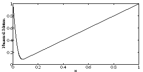
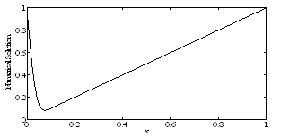
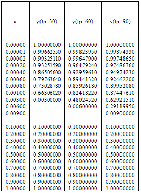
  The numerical results are given in tables 1 & 2 for τ=0.5 and ε=10–3 , ε=10–4 respectively. For τ=1.5 andτ=2.5, the inner solution is plotted in graphs and shown in fig. 1 to fig 4 for ε=10–3 , ε=10–4 respectively.
Table 1. Numerical results of Example 1 for ε=10–3, τ=0.5.
 |
| |
|
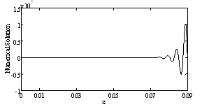 | Figure 1. Inner solution of Example 1 for ε=10–3, τ=1.5. |
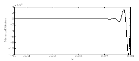 | Figure 2. Inner solution of Example 1 for ε=10–3, τ=2.5. |
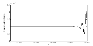 | Figure 3. Inner solution of Example 1 for ε=10–4, τ=1.5. |
 | Figure 4. Inner solution of Example 1 for ε=10–4, τ=2.5. |
Table 2. Numerical results of Example 1 for ε=10–4, τ=0.5.
 |
| |
|
Example 2[1, p.e1921]:  with the interval and boundary conditions
  The solution at the cutting point is given by the reduced problem solution
  where
where  and
and  and hence
  The linearized form of the given nonlinear equation by quasilinearization method is
  with the conditions
  ,
,  The inner region problem is given by
  ,
, under the conditions
 ,
,  The outer region problem is given by
 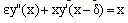 ,
,  under the conditions
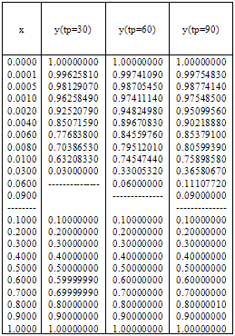
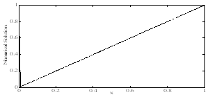
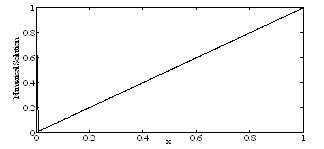
  The numerical results are given in tables 3 & 4 for τ=0.5 and ε=10–3 , ε=10–4 respectively. For τ=1.5 and τ=2.5, the numerical solution is plotted in graphs and shown in fig. 5 to fig. 8 for ε=10–3 , ε=10–4 respectively.
 Table 3. Numerical results of Example 2 for ε=10-3, τ=0.5.
 |
| |
|
 | Figure 5. Numerical solution of Example 2 for ε=10–3, τ=1.5. |
 | Figure 6. Numerical solution of Example 2 for ε=10–3, τ=2.5. |
 | Figure 7. Numerical solution of Example 2 for ε=10–4, τ=1.5. |
 | Figure 8. Numerical solution of Example 2 for ε=10–4, τ=2.5. |
Table 4. Numerical results of Example 2 for ε=10-4, τ=0.5.
 |
| |
|
5. Conclusions
In order to know the behavior of the solution of the singularly perturbed differential-difference equations in the boundary layer region, it is always suggestive to divide the original problem into two problems namely the inner region problem and the outer region problem and solve them separately. We have presented a numerical patching technique for solving singularly perturbed nonlinear differential-difference equations with the boundary layer at one end point. The original nonlinear boundary value problem is linearized using quasilinearization. Then it is divided into two problems namely inner region problem and outer region problem. The boundary condition at the cutting point is obtained from the theory of singular perturbations. A new inner region problem is constructed and solved by using upwind finite difference scheme. The outer region problem is solved by Taylor polynomial approach. We have implemented the present method on two nonlinear examples exhibiting a left end boundary layer. The proposed method is iterative on the cutting point. The process is to be repeated for various choices of the cutting point, until the solution profiles do not differ materially from iteration to iteration. Numerical results are presented in tables. It can be observed from the tables that the present method approximates the solution available in the literature as well.
ACKNOWLEDGMENTS
The authors wish to thank the Department of Science & Technology, Government of India, for their financial support under the project No. SR/S4/MS: 598/09.
References
| [1] | Mohan K. Kadalbajoo and Kapil K. Sharma, Numerical treatment for singularly perturbed nonlinear differential difference equations with negative shift, Nonlinear Analysis 63 (2005) e1909-e1924 |
| [2] | Mohan K. Kadalbajoo and Devendra Kumar, A computational method for singularly perturbed nonlinear differential-difference equations with small shift, Applied Mathematical Modelling 34 (2010) 2584-2596 |
| [3] | Mohan K. Kadalbajoo and Kapil K. Sharma, A numerical method based on finite difference for boundary value problems for singularly perturbed delay differential equations, Applied Mathematics and Computation 197 (2008) 692-707 |
| [4] | C.G. Lange and R.M. Miura, Singular perturbation analysis of boundary-value problems for differential difference equations, IV, a nonlinear example with layer behavior, Stud. Appl. Math. 84 (1991) 231-273 |
| [5] | C.G. Lange and R.M. Miura, Singular perturbation analysis of boundary-value problems for differential difference equations. V. Small shifts with layer behavior, SIAM Journal on Applied Mathematics 54 (1994) 249–272 |
| [6] | Mustafa Gulsu and Mehmet Sezer, A Taylor polynomial approach for solving differential- difference equations, Journal of Computational and Applied Mathematics 186 (2006) 349 - 364 |
| [7] | E.P. Doolan, J.J.H. Miller, W.H.A. Schilders, Uniform Numerical Methods for Problems with Initial and Boundary Layers, Boole Press, Dublin, 1980 |
| [8] | R.E. Bellman, R.E. Kalaba, Quasilinearization and Nonlinear Boundary–Value Problems, American Elsevier, New York, 1965 |
| [9] | F.A. Howes, Singular Perturbations and Differential Inequalities, vol. 168, Memoirs of the American Mathematical Society, Providence, RI, 1976 |
| [10] | Y. Kuang, Delay Differential equations with applications in population dynamics, Academic Press, 1993 |
| [11] | R.B. Stein, A theoretical analysis of neuronal variability, Biophysical Journal 5 (1965) 173-194 |
| [12] | L .E. El’sgol’ts, Qualitative Methods in Mathematical Analyses, Translations of Mathematical Monographs 12, American mathematical society, Providence, RI, 1964 |
 Abstract
 Reference
 Full-Text PDF
 Full-Text HTML