1. Introduction

The use of networks transporting probabilities began with the geneticist Sewall Wright in the beginning of the 20th century (1921). Since then their use had different forms in several areas like social sciences and economy – in which the used models are, in general, linear named Path Diagrams or Structural Equations Models (SEM), and in artificial intelligence – usually non-linear models named Bayesian networks also called Probabilistic Expert Systems (PES).

Bayesian networks are graphical structures for representing the probabilistic relationships among a large number of variables and for doing probabilistic inference with those variables,[1]. Before approaching the use of Bayesian networks to the interest problems some aspects of PES in connection with uncertainty problems must be studied, see for instance[2].

2. Objectives

A crime has been committed, and two persons were murdered, V₁ and V₂. At the crime scene two different mixture traces were found: T₁ in the toilet and T₂ in the victims' car. S₂ is a potential suspect. S₂'s DNA profile was measured and found to be compatible with the mixture traces.

Accepting that there was a fight during the assault that produced some material, it is obvious that the individual who perpetrated the crime could left some of his/her material in some but not in the whole traces. The non-DNA evidence indicates the possibility that two people were involved in the crime.

In[3] it is described a new approach to the problems mentioned in 1. The construction and use of Bayesian networks to analyse complex problems of forensic identification inference was initially done there followed by [4-6,7] among others.

The advances achieved in the forensic biology have certainly encouraged the interest in problems of forensic identification, also allowing a much more rigorous treatment of the problems in analysis. That is the case of problems of DNA mixtures –[6,7].

One of the complexities in the interpretation of the mixture traces is assigning the number of contributors to the mixture. In general, the trace suggests a lower bound for the total number of contributors but no upper bound.[5] gave a useful low upper bound on the number of contributors worth considering.

In what follows it is described a complex mixture case, related with the former crime scene, and presented the data to be considered in the analysis. After formulating the hypotheses the analysis is performed for one marker considering the information from one trace. Then the two traces are considered and finally the analysis is generalized considering two mixture traces and the three markers.

3. Methods

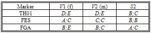
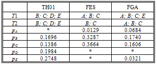
To summarize the evidence is presented in Table 1 the DNA profiles of the victims' and the suspect, S₂. In Table 2 the profiling results for the mixtures traces (T₁ and T₂), for the STR markers studied, respectively, and the allele frequencies for each marker are presented.

The traces contain biological material that must belong to some person other than the two victims.

The allele frequencies used in this work are the Portuguese population frequencies collected in the worldwide database “The Distribution of Human DNA-PCR Polymorphisms”, since the case mentioned took place in Portugal.

Table 1. Two victims and suspect DNA profiles

It is natural to consider that the crime traces can contain DNA from up to three unknown contributors, in addition to the victims and/or the suspect.

Table 2. DNA mixture traces and allele frequencies1

If the DNA from S₂ is present in at least one of the traces this will place him at the crime scene and consequently as one of the possible perpetrators. Consideration of whether or not the suspect was a contributor to any of the mixture traces will give a measure of the evidence strength.

Hypotheses

The court has to determine if the suspect is or is not guilty. These are described as the level III, or offence, propositions. However the forensic scientist does not typically address such propositions. In this case it appears more appropriate to address source level propositions.

Hypotheses to be addressed:

H₁: S₂ is one of the contributors to T₁ but not T₂.

H₂: S₂ is one of the contributors to T₂ but not T₁.

H₃: S₂ is one of the contributors to both T₁ and T₂.

H₄: S₂ did not contribute to trace T₁ or T₂.

What interests is to measure:

where is the vector comprising the profiles observed of the traces found at the crime scene: the victims’ and the suspect profiles. This is equivalent to

One mixture trace and a single marker

The network for one trace and a single marker follows[7], Figure 4 section 3.2, an OOBN version considering up to three unknown contributors Figure 1, marker network. Here it is presented the network for the marker, FES².

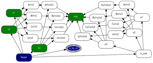Figure 1. Marker network

Two mixture traces and a single marker

As described above there were two different traces at the crime scene. So it is necessary to combine the information from both traces. To do so define an instance combine, Figure 2. This instance has as parents the output nodes vi_by_s2 of the instance marker for trace T₁ and trace T₂. The node T₁_T₂ combines the results obtained in the parent instances for node vi_by_s2 expressing the result values of the one-to-one correspondence with the eight joint configurations of its parents nodes for the considered marker.

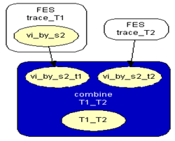
Figure 2. Combine network

Therefore, the node T₁_T₂ takes values 0, 1, 2, 3 corresponding to the hypothesis H₄, H₁, H₂ and H₃, respectively. T₁_T₂ is 0 if vi_by_s2 is less than 4 in T₁ and T₂; assumes value 1 if vi_by_s2 is equal to 4 or more in T₁ and less than 4 in T₂; takes value 2 if vi_by_s2 is less than 4 in T₁ and equal to 4 or more in T₂; and is 3 if vi_by_s2 is equal to 4 or more in both T₁ and T₂. In the start a uniform prior distribution for node T₁_T₂ is assumed.

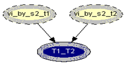
Figure 3. Combine_T1_T2 network

Now it is possible to put the networks for each trace together and compute the interest information, Figure 3. The instances FES trace_t1 and FES trace_t2 are of class marker in which all the individuals in any of the networks have the same structure (individual). Its differentiation is made when the evidence is inserted.

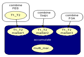
4. Results

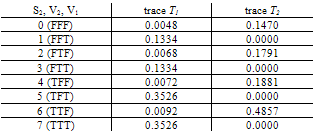
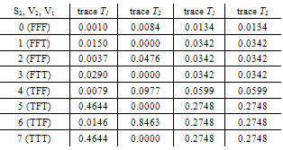
When combining the two traces, in order to obtain a measure of the evidential weight associated with the possible presence of genetical material from the suspect in the traces found at the crime scene, the results listed in the Tables below are got. For marker FES with different mixture traces it is obtained:

Table 3. Results of the node vi_by_s2

Where the state 0 corresponds to s2_in_mix? = False, v2_in_mix? =False and v1_in_mix? = False (FFF), and for simplicity the state 0 is read as S₂; V₂; V₁ = FFF.

In Table 4 it is shown the combined information for the two traces for marker FES.

Table 4. Results for the node T1_T2

Thus,

.

Generalization: two mixture traces and three markers

Given the results obtained for one marker it is necessary to extend the reasoning in order to consider the information for the three markers, FES, TH01 and FGA.

The instances combine_T₁_T₂ express the results for each marker accounting for the information for the two traces. The node T₁_T₂ in each of these instances computes the results for each marker. The respective tables, similar to Table 4, can be extracted for the other two markers.

The instance accumulate having as inputs the output nodes of the instances combine T1_T2, with the results of each marker, incorporates the information for the two traces obtained separately, Figure 4. The node multi_markers combines the information from the different instances combine_T1_T2, i.e., multi_markers gives the results synthesizing the results of T1_T2 for the three markers. The node multi_markers with states 0, 1, 2 and 3 assumes the state 0 if all the input nodes are 0. Takes value 1 if all the input nodes are 1 or at least one of the input nodes has state 1 and the others have the state 0³ . The node multi markers is 2 if all the input nodes have state 2 or this state 2 is combined between the states 0 and 2 of the input nodes. The node assumes state 3 if all the input nodes have state 3 or if the inputs are combining state 0, state 1 and state 2.

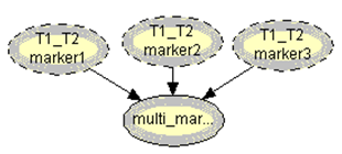Figure 4. Accumulate network

Joining the networks for the three markers, each of which accounts for the two traces, it is obtained the accumulate_three_markers network, Figure 5.

Figure 5. Accumulate three markers network

Tables 5 and 6 display the results for the marker FGA and TH01 and the cumulative result for all three markers, rescaled to sum up to 1. This aims at the question of interest.

Table 5. Results for the eight configurations for markers FGA and TH01

Table 6. Results for the node T1_T2 for markers FGA and TH01

Therefore,

5. Discussion

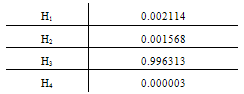
When the whole information for the two traces on the three markers is taken into account a very significant value for the interest quantity is obtained.

The use of DNA evidence analysis is commonly accepted nowadays in the whole courts. However, the presentation, interpretation and evaluation of this type of evidence sometimes raise some problems. And it is far the day when a total incorporation of this kind of evidence is achieved, although in some cases it has been decisive for the conviction or absolution of the individuals. This is already a good support for justice.

6. Conclusions

The statistical treatment of criminal evidence has raised new challenges to those that have to decide, in the basis of the presented results. Independently of the methodology used, the great difficulty inhabits in the interpretation of the evidence, which is summarized in a number – what does that value means?

In the most complex problems, as the mentioned ones, the use of Bayesian networks for the analysis and interpretation of the evidence can be of great help. In a Bayesian network the complex inter-relations between the variables are transformed into modular units.

This technology – which use is everyday more common in different areas – supplies, as a support to the decision, a number. It does not give the decision; it is a decision support instrument. Consequently it is important that the legal system knows how to evaluate and interpret correctly the information contained in it. However, there is still much to do.

Notes

1. The use of * refers values that are of no concern in the analysis.

2. The marker networks differ only in the number of alleles to consider, whether it is the space of states of the nodes referring the alleles or in the presence of one more allele to consider in the network. Since Hugin software does not allow modification of the state of a node in order to reuse a network, for markers TH01 and FGA a codification in the space of states of the node gene was performed and put it in accordance with the alleles of each marker under consideration so that it could used the same network.

3. e.g., multi markers=1 if T1_T2 =1 for marker1, marker2 and marker3; or T1_T2 =1 for marker1 and marker2 and T1_T2 =0 for marker3; or T1_T2 =1 for marker1 and marker3 and T1_T2 =0 for marker2; or T1_T2 =1 for marker2 and marker3 and T1_T2 =0 for marker1; or T1_T2 =1 for marker1 and T1_T2 =0 for marker2 and marker3; or T1_T2 =1 for marker2 and T1_T2 =0 for marker1 and marker3; or T1_T2 =1 for marker3 and T1_T2 =0 for marker1 and marker2.

ACKNOWLEDGEMENTS

This work was financially supported by FCT through the Strategic Project PEst-OE/EGE/UI0315/2011.