José María Mínguez
Dpto. de Física Aplicada II, Universidad de Bilbao, Bilbao, 48930, Spain
Correspondence to: José María Mínguez , Dpto. de Física Aplicada II, Universidad de Bilbao, Bilbao, 48930, Spain.
| Email: |  |
Copyright © 2012 Scientific & Academic Publishing. All Rights Reserved.
Abstract
This short paper deals with the implicit function  , X,Y > 0, and shows surprinsingly how accurately it is equivalent to another very much simpler and explicit function.
Keywords:
Power Exponential Function, Equivalent Function, Approximation
1. Introduction
The literature devoted to the equation  ,
,  , is really limited. From[1] we know that L. Euler treated it and gave a parametric representation, from which the rational solutions were drawn. He also deduced the existence of the two asymptotes (
 and
and  ) to the curve. The same paper gives notice that also Daniel Bernouilli found the rational solutions. Later E. J. Moulton[2] writes a discussion of the curve defined by
  ,
,  , and recently Y. S. Kupitz and H. Martini[3] demonstrate the following two propositions: (1) There is a non-trivial solution
  to the equation
  ,
,  , if and only if
  , and for such a
  the solution is unique, and (2) The only non-trivial integer solutions to the equation
  ,
,  , are (2, 4) and (4, 2).Recently this function has also focussed the attention of mathematicians[5,6], although little has been added to its knowledge and development.In brief, it is well known that the implicit power- exponential function
 | (1) |
admits the trivial solution, which will be named as solution (A), | (2) |
and another solution (B), which may be found either by successive iterations or by using some software, like Mathematica[4], in a computer.Obviously, solution (B) is symmetrical with respect to the straight line defined by solution (A).
2. Non-Trivial Solution (B)
To find out the solution (B) one can proceed as follows:From (1)  | (3) |
 | (4) |
 | (5) |
 | (6) |
 | (7) |
And, | (8) |
being ProductLog[z] the function which gives the principal solution for w in | (9) |
as defined and tabulated by Mathematica.Then solution (B) may be tabulated from | (10) |
Both, equation (10) and direct iterations, yield the results shown in Table I, by means of which figure 1 represents the solution (B) (continuous line), together with solution (A) (discontinuous line).
3. Equivalent Function
Figure 1 shows at first glance that the function YB looks very close to the hyperbola | (11) |
which, by the way, also admits the integer solutions (2, 4) and (4, 2) as equation (1).In order to analyse how close the function (11) is to the original function YB, a third column (YH1) is added in Table I, showing | (12) |
as given by (11), whereas the fifth column shows the distance YH1 – YB.Then, accounting for the fact that the curve  also goes through the point (e, e), the hyperbola
  | (13) |
is considered too and  | (14) |
as given by (13), is shown in the fourth column of table 1, whereas the distance YH2 - YB appears in the sixth column. | | X | YB | YH1 | YH2 | YH1-YB | YH2-YB | | e | e | 2.7459 | 2.7183 | 0.0276 | 0.0000 | | 2.8 | 2.6405 | 2.6667 | 2.6403 | 0.0262 | -0.0002 | | 2.9 | 2.5548 | 2.5790 | 2.5539 | 0.0242 | -0.0009 | | 3.0 | 2.4781 | 2.5000 | 2.4763 | 0.0219 | -0.0018 | | 3.5 | 2.1897 | 2.2000 | 2.1810 | 0.0103 | -0.0087 | | 4.0 | 2.0000 | 2.0000 | 1.9842 | 0.0000 | -0.0158 | | 4.5 | 1.8655 | 1.8571 | 1.8436 | -0.0084 | -0.0219 | | 5.0 | 1.7649 | 1.7500 | 1.7381 | -0.0149 | -0.0268 | | 6.0 | 1.6242 | 1.6000 | 1.5905 | -0.0242 | -0.0337 | | 7.0 | 1.5301 | 1.5000 | 1.4921 | -0.0301 | -0.0380 | | 8.0 | 1.4625 | 1.4286 | 1.4218 | -0.0339 | -0.0407 | | 9.0 | 1.4114 | 1.3750 | 1.3691 | -0.0364 | -0.0423 | | 10.0 | 1.3713 | 1.3333 | 1.3281 | -0.0380 | -0.0432 | | 12.0 | 1.3122 | 1.2727 | 1.2684 | -0.0395 | -0.0438 | | 14.0 | 1.2707 | 1.2308 | 1.2271 | -0.0399 | -0.0436 | | 16.0 | 1.2396 | 1.2000 | 1.1968 | -0.0396 | -0.0428 | | 18.0 | 1.2155 | 1.1765 | 1.1737 | -0.0390 | -0.0418 | | 20.0 | 1.1962 | 1.1579 | 1.1554 | -0.0383 | -0.0408 | | 25.0 | 1.1613 | 1.1250 | 1.1230 | -0.0363 | -0.0383 | | 30.0 | 1.1377 | 1.1034 | 1.1018 | -0.0343 | -0-0359 | | 35.0 | 1.1206 | 1.0882 | 1.0868 | -0.0324 | -0.0338 | | 40.0 | 1.1075 | 1.0769 | 1.0757 | -0.0306 | -0.0318 | | 45.0 | 1.0973 | 1.0682 | 1.0671 | -0.0291 | -0.0302 | | 50.0 | 1.0889 | 1.0612 | 1.0603 | -0.0277 | -0.0286 | | 60.0 | 1.0762 | 1.0508 | 1.0500 | -0.0254 | -0.0262 | | 70.0 | 1.0669 | 1.0435 | 1.0428 | -0.0234 | -0.0241 | | 80.0 | 1.0598 | 1.0380 | 1.0374 | -0.0218 | -0.0224 | | 90.0 | 1.0541 | 1.0337 | 1.0332 | -0.0204 | -0.0209 | | 100.0 | 1.0495 | 1.0303 | 1.0298 | -0.0192 | -0.0197 | | 125.0 | 1.0410 | 1.0242 | 1.0238 | -0.0168 | -0.0172 | | 150.0 | 1.0352 | 1.0201 | 1.0198 | -0.0151 | -0.0154 | | 175.0 | 1.0309 | 1.0172 | 1.0170 | -0.0137 | -0.0139 | | 200.0 | 1.0276 | 1.0151 | 1.0148 | -0.0125 | -0.0128 | | 250.0 | 1.0228 | 1.0120 | 1.0119 | -0.0108 | -0.0109 | | 300.0 | 1.0196 | 1.0100 | 1.0099 | -0.0096 | -0.0097 | | 400.0 | 1.0153 | 1.0075 | 1.0074 | -0.0078 | -0.0079 | | 500.0 | 1.0127 | 1.0060 | 1.0059 | -0.0067 | -0.0068 |
|
|
Thus, direct reading of table I shows that the hyperbola (11) is closer to YB than the hyperbola (13), and that | (15) |
for two reasons: 1) this value is not reached before  , and 2) for
  and onwards the distance between YB and the asymptote
  , as well as between YH1 and the same asymptote, is less than 0.04, which implies (15).In fact, in figure 1 the points representing YH1 are plotted over the curve YB and the closeness is very evident.
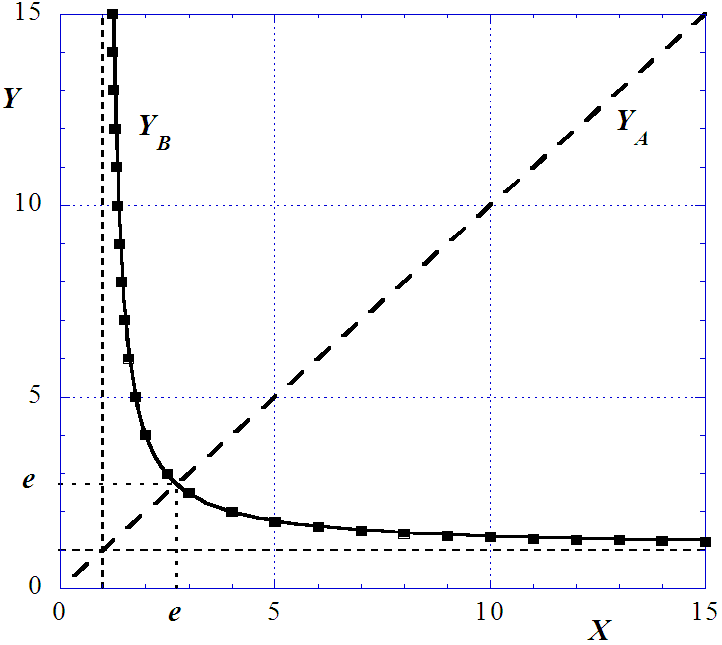 | Figure 1. Trivial solution (A) (discontinuous straight line) and solution (B) (full line curve). Overlapping the curve the dots representing the equivalent hyperbolic function |
4. Conclusions
The little difference between the two functions YH1 and YB, which remains always under 0.04, means that the much simpler hyperbola given by equation (11) is a very good approximation to the implicit power-exponential function defined by equation (1).
References
| [1] | R. C. Archivald, “Problem notes, No. , Amer. Math. Monthly, vol. 28, pp. 141-143, 1921 |
| [2] | E. J. Moulton, “The real function defined by x y = yx “, Amer. Math. Monthly, vol. 23, pp. 233-237, 1916 |
| [3] | Y. S. Kupitz, and H. Martini, C. “On the equation xy = yx ”, Elemente der Mathematik, vol. 55, pp. 95–101, 2000 |
| [4] | Mathematica, Trade Mark. Wolfram Research, Inc., |
| [5] | Mitteldorf, “Solutions to x y = yx “ [on line]. Available from: http://mathforum.org/library/drmath/view/53229.html (accessed November 2011) |
| [6] | Vogler, “Solving the equation x y = yx “[on line]. Available from: http://mathforum.org/library/drmath/view/66166.html (accessed November 2011) |
 Abstract
 Reference
 Full-Text PDF
 Full-Text HTML