-
Paper Information
- Next Paper
- Previous Paper
- Paper Submission
-
Journal Information
- About This Journal
- Editorial Board
- Current Issue
- Archive
- Author Guidelines
- Contact Us
Applied Mathematics
p-ISSN: 2163-1409 e-ISSN: 2163-1425
2011; 1(2): 90-98
doi: 10.5923/j.am.20110102.15
Conjugate Transient Free Convective Heat Transfer from a Vertical Slender Hollow Cylinder with Heat Generation Effect
 Abstract
 Reference
 Full-Text PDF
 Full-Text HTML
H. P. Rani , G Janardhana Reddy
Department of Mathematics, National Institute of Technology, Warangal, 506004, India
Correspondence to: H. P. Rani , Department of Mathematics, National Institute of Technology, Warangal, 506004, India.
| Email: |  |
Copyright © 2012 Scientific & Academic Publishing. All Rights Reserved.
Numerical analysis is performed to study the conjugate heat transfer and heat generation effects on the transient free convective boundary layer flow over a vertical slender hollow circular cylinder with the inner surface at a constant temperature. A set of non-dimensional governing equations namely, the continuity, momentum and energy equations is derived and these equations are unsteady non-linear and coupled. As there is no analytical or direct numerical method available to solve these equations, they are solved using the CFD techniques. An unconditionally stable Crank-Nicolson type of implicit finite difference scheme is employed to obtain the discretized forms of the governing equations. The discretized equations are solved using the tridiagonal algorithm. Numerical results for the transient velocity and temperature profiles, average skin-friction coefficient and average Nusselt number are shown graphically. In all these profiles it is observed that the time required to reach the steady-state increases as the conjugate-conduction parameter or heat generation parameter increases.
Keywords: Conjugate Heat Transfer, Heat Generation, Natural Convection, Vertical Slender Hollow Cylinder, Finite Difference Method
Cite this paper: H. P. Rani , G Janardhana Reddy , "Conjugate Transient Free Convective Heat Transfer from a Vertical Slender Hollow Cylinder with Heat Generation Effect", Applied Mathematics, Vol. 1 No. 2, 2011, pp. 90-98. doi: 10.5923/j.am.20110102.15.
Article Outline
1. Introduction
- Transient natural convection flow of a viscous incompressible fluid with heat transfer is an important problem relevant to many engineering applications. They have wide applications in Science and Technology. These types of problems are commonly encountered in start-up of a chemical reactor and emergency cooling of a nuclear fuel element. In the case of power or pump failure, similar conditions may arise for devices cooled by forced circulation, as in the core of a nuclear reactor. In the glass and polymer industries, hot filaments, which are considered as a vertical cylinder, are cooled as they pass through the surrounding environment. The exact solution for these types of non-linear problems is still out of reach. Sparrow and Gregg[1] provided the first approximate solution for the laminar buoyant flow of air bathing a vertical cylinder heated with a prescribed surface temperature, by applying the similarity method and power series expansion. Minkowycz and Sparrow[2] obtained the solution for the same problem using the non-similarity method. While Fujii and Uehara[3] analyzed the local heat transfer results for arbitrary Prandtl numbers.Lee et al.[4] investigated the similar problem along slender vertical cylinders and needles for the power-law variation in the wall temperature. In general, Bottemanne 5] studied the combined effect of heat and mass transfer in the steady laminar boundary layer of a vertical cylinder for air and water vapour. Recently, Rani and Kim 6] investigated the unsteady effects for the similar problem with temperature dependent viscosity.It can be observed that in the previous investigations the wall conduction resistance in the case of convective heat transfer between a solid cylinder wall and a fluid flow is generally neglected i.e. the wall is assumed to be very thin and there is no conduction from the cylinder wall. But in many practical problems the information on the interfacial temperature is essential because the heat transfer characteristics are mainly determined by the temperature differences between the bulk flow and the interface. In order to take account of physical reality, there has been a proclivity to move away from considering idealized mathematical problems in which the bounding wall is considered to be infinitesimally thin. Thus the conduction in solid wall and the convection in the fluid should be determined simultaneously. This type of convective heat transfer is referred to as a conjugate heat transfer (CHT) process and it arises due to the finite thickness of the wall. These type of problems are usually referred to as conjugate heat transfer problems, and they have many practical applications, particularly those related to energy conservation in buildings, cold storage installations and cryogenic applications, such as medical and space technology. The early theoretical and experimental work of CHT problem for a viscous fluid has been reviewed by Gdalevich and Fertman[7] and Miyamoto et al.[8]. Gdalevich and Fertman[7] gave review about the conjugate problems of free convection with the details about the methods, specifics and principal results. They stated conclusively that the use of numerical methods for solving the initial system of governing partial differential equations, such as finite difference method, is evidently the most promising in the studies of conjugate free convection. Char et al.[9] employed the cubic spline collocation numerical method to analyze the CHT in the laminar boundary layer on a continuous, moving plate. Pop et al.[10] presented a detailed numerical study of the conjugate mixed convection flow along a vertical flat plate. Pop and Na[11] reported a numerical study of the steady conjugate free convection over a vertical slender, hollow circular cylinder with the inner surface at a constant temperature and embedded in a porous medium. Recently, Kaya[12] studied the effects of buoyancy and CHT on non-Darcy mixed convection about a vertical slender hollow cylinder embedded in a porous medium with high porosity.The CHT problems associated with the heat generating plate were studied by Karvinen[13], Sparrow et al.[14] and Garg et al.[15] using an approximate method. Analytical and numerical solutions were performed by Vynnycky et al.[16] for the CHT problem associated with the forced convection flow over a conducting slab sited in an aligned uniform stream. Vajravelu and Hadjinicolaou[17] analyzed the heat transfer behavior within the boundary layer of a viscous fluid over a stretching sheet with viscous dissipation and internal heat generation. Moreover, effects of heat generation/absorption and thermophoresis on hydromagnetic flow along a flat plate were studied by Chamkha and Camille[18].From the above studies, it can be noted that the CHT on the unsteady natural convective flow of a viscous incompressible fluid over a vertical cylinder with heat generation has received very scant attention in the literature. Hence, in the present investigation our attention is focused on the effect of heat generation on the coupling of conduction inside and the laminar natural convection flow over the outside surface of a vertical slender hollow cylinder. The temperature of the inner surface of the cylinder is kept at a constant value which is higher than the ambient fluid temperature and the temperature of the outer surface is determined by the conjugate solution of the steady-state energy equation of the solid and the boundary layer equations of the fluid flow. The governing equations are solved numerically by the implicit finite difference method to obtain the transient velocity and temperature profiles, coefficient of skin-friction and heat transfer rate for different values of conjugate-conduction and heat generation parameters.In section 2, a detailed description about the formulation of the problem is given. Also, the governing equations, such as mass, momentum and energy equations of an incompressible fluid flow past a vertical cylinder are derived and non-dimensionalized. In section 3, the details about the grid generation and numerical methods for solving the above governing equations are given. In section 4, transient two-dimensional velocity and temperature profiles, average skin-friction coefficient and heat transfer rate are analyzed. Finally, the concluding remarks are made in section 5.
2. Mathematical Formulation
- An unsteady two-dimensional laminar natural convection boundary layer flow of a viscous incompressible fluid past a vertical slender hollow cylinder of length l and outer radius
 is considered as shown in Fig. 1. The x-axis is measured vertically upward along the axis of the cylinder. The origin of x is taken to be at the leading edge of the cylinder, where the boundary layer thickness is zero. The radial coordinate, r, is measured perpendicular to the axis of the cylinder. The surrounding stationary fluid temperature is assumed to be of ambient temperature (
 ). The temperature of the inside surface of the cylinder is maintained at a constant temperature of
  , where
  . Initially, i.e., at time
  it is assumed that the outer surface of the cylinder and the fluid are of the same temperature
  . As time increases (
 ), the temperature of the outer surface of the cylinder is raised to the solid-fluid interface temperature
  and maintained at the same level for all time
  . This temperature
  is determined by the conjugate solution of the steady-state energy equation of the solid and the boundary layer equations of the fluid flow and is discussed elsewhere. It is assumed that the effect of viscous dissipation is negligible in the energy equation. Under these assumptions, the boundary layer equations of mass, momentum and energy with Boussinesq's approximation are as follows:
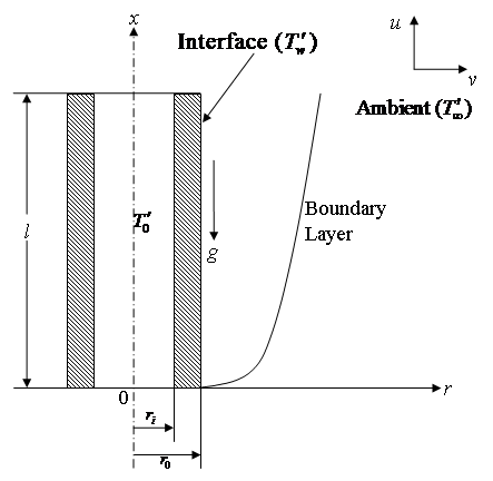 | Figure 1. Schematic of the investigated problem |
 | (1) |
 | (2) |
 | (3) |
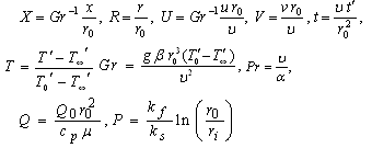
 ,
,  being a constant, represents the amount of generated or absorbed heat per unit volume. Heat is generated or absorbed from the source term according as
 is positive or negative.The corresponding initial and boundary conditions are given by
 | (4) |
 is the unknown solid-fluid interface temperature and is determined as follows:To predict the outer surface temperature of the cylinder
  , an additional governing equation is required for the slender hollow cylinder based on the simplification that the wall of cylinder steady transfers its heat to the surrounding fluid. Since the outer radius of the hollow cylinder,
  , is small compared to its length, l, the axial conduction term in the heat conduction equation of the cylinder can be omitted. The governing equation for the temperature distribution within the slender hollow circular cylinder is given by Chang 20] as follows:
 | (5) |
 | (6) |
 | (7) |
 | (8) |
 at the interface is given by
 | (9) |
 | (10) |
 | (11) |
 | (12) |
 | (13) |
 | (14) |
3. Numerical Solution
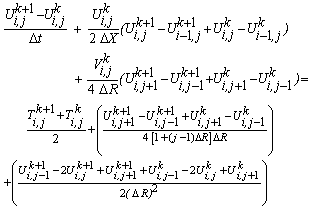
- In order to solve the unsteady coupled non-linear governing Eqs. (11)-(13) an implicit finite difference scheme of Crank-Nicolson type has been employed. The finite difference equations corresponding to Eqs. (11) - (13) are as follows:
 | (15) |
 | (16) |
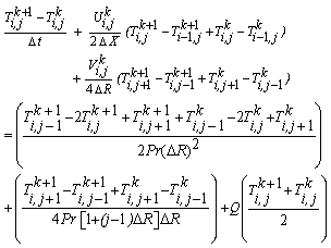 | (17) |
 which lies very far from the momentum and energy boundary layers. In the above Eqs. (15)-(17) the subscripts i and j designate the grid points along the X and R coordinates, respectively, where X = i ∆X and R = 1 + (j -1) ∆R and the superscript k designates a value of the time t (= k ∆t), with ∆X, ∆R and ∆t the mesh size in the X, R and t axes, respectively. In order to obtain an economical and reliable grid system for the computations, a grid independent test has been performed which is shown in Fig. 2. The steady-state velocity and temperature values obtained with the grid system of 100 × 500 differ in the second decimal place from those with the grid system of 50 × 250, and in the fifth decimal place from those with the grid system of 200 × 1000. Hence, the grid system of 100 × 500 has been selected for all subsequent analyses, with mesh size in X and R direction are taken as 0.01 and 0.03, respectively. Also, the time step size dependency has been carried out, from which 0.01 yielded a reliable result. From the initial conditions given in Eq. (14), the values of velocity U, V and temperature T are known at time t = 0, then the values of T, U and V at the next time step can be calculated. Generally, when the above variables are known at t = k ∆t, the variables at t = (k + 1) ∆t are calculated as follows. The finite difference Eqs. (16) and (17) at every internal nodal point on a particular i-level constitute a tridiagonal system of equations. Such a system of equations is solved by the Thomas algorithm (Carnahan et al. 21]). At first, the temperature T is calculated from Eq. (17) at every j nodal point on a particular i-level at the (k + 1)th time step. By making use of these known values of T, the velocity U at the (k+1)th time step is calculated from Eq. (16) in a similar manner. Thus, the values of T and U are known at a particular i-level. Then the velocity V is calculated from Eq. (15) explicitly. This process is repeated for the consecutive i-levels; thus the values of T, U and V are known at all grid points in the rectangular region at the (k + 1)th time step. This iterative procedure is repeated for many time steps until the steady-state solution is reached. The steady-state solution is assumed to have been reached when the absolute difference between the values of velocity as well as temperature at two consecutive time steps is less than
  at all grid points. The truncation error in the employed finite difference approximation is
  and tends to zero as ∆X, ∆R and ∆t → 0. Hence the system is compatible. Also, this finite difference scheme is unconditionally stable and therefore, stability and compatibility ensure convergence.
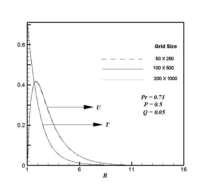 | Figure 2. Grid independent test for velocity and temperature profiles |
4. Results and Discussion
- To validate the current numerical procedure, the present simulated velocity and temperature profiles are compared with those of the available steady-state, isothermal results of Lee et al. 4] for air (Pr = 0.7) without conduction and heat generating effects i.e., P = 0.0 and Q = 0.0, as there are no experimental or analytical studies available to compare with the present problem. The current results are found to be in good agreement with the previous results available in literature as shown in Fig. 3.The simulated results are presented to outline the general physics involved in the effects of different Q ( = 0.01, 0.05, 0.08 and 0.10) 19] and P ( = 0.1, 0.5, 1.0 and 2.0) 11] with fixed Pr [ = 0.71 (air)] on the transient velocity and temperature profiles. The simulated transient behaviour of the dimensionless velocity, temperature, average skin-friction coefficient and heat transfer rate are discussed in detail in the succeeding subsections.
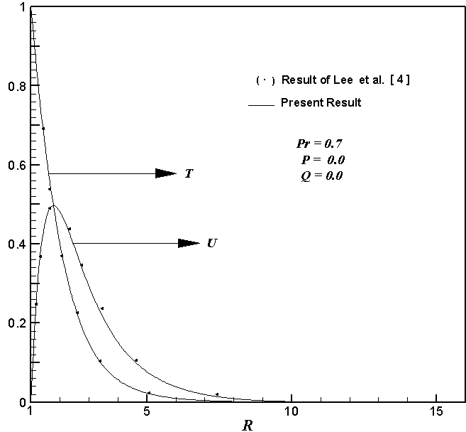 | Figure 3. Comparison of the velocity and temperature profiles |
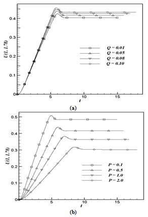 | Figure 4. The simulated transient velocity at (1, 1.78) for (a) variation of Q with fixed P = 0.5; (b) variation of P with fixed Q = 0.05 |
4.1. Velocity
- The simulated transient velocity (U) at (1, 1.78) for different values of heat generation parameter Q and conjugate-conduction parameter P against t is shown graphically in Fig. 4. Fig. 4a shows the variation of Q with fixed P = 0.5 and Fig. 4b for the variation of P with fixed Q = 0.05. From Figs. 4a and 4b it is observed that the velocity increases with time, reaches a temporal maximum, then decreases and at last reaches the asymptotic steady-state. For example, in Fig. 4a when Q = 0.01, the velocity increases with time monotonically from zero and reaches the temporal maximum, then slightly decreases with time and becomes asymptotically steady. It is observed that at the very early time (i.e., t < < 1), the heat transfer is dominated by conduction. Shortly later, there exists a period when the heat transfer rate is influenced by the effect of convection with the increasing upward velocities along the time. When this transient period is almost ending and just before the steady-state is about to be reached, there exist overshoots of the velocities. From Figs. 5a and 5b it can be observed that velocity profiles reach their maximum value approximately at (1, 1.78). Similarly, the velocity at other locations also exhibits somewhat similar transient behaviour. As noted in Fig. 4a, the magnitude of this overshoot of the velocities increases as Q is increased, since with the increasing Q the velocity diffusion is decreased (refer Eq. (12)). Hence, there is a high resistance to the fluid flow in the region of the temporal maximum of velocity. The time needed to reach the temporal maximum of the velocity increases as Q increases. It is also noticed that for small values of Q the temporal maximum is reached at early times. For all values of P, Figure 4b reveals that it has the same trend as the transient behaviour with respect to Q shown in Fig. 4a, but the temporal maximum of velocity decreases as P increases. In association with the transient characteristics of the velocity, similar trends of the temperature fluctuation can be observed and will be described in Fig. 6.Figure 5 shows the simulated steady-state velocity profiles against the R at X = 1.0 for different values of Q and P. Fig. 5a shows the variation of Q with fixed P = 0.5 and Fig. 5b for the variation of P with fixed Q = 0.05. From these figures it is observed that the velocity profile start with the value zero at the wall, reach their maximum and then monotonically decrease to zero along the radial coordinate for all t. Also it is observed that in the vicinity of the wall the magnitude of the axial velocity is rapidly increasing as R increases from Rmin (=1). From Fig. 5a it is observed that the velocity increases with the increasing values of Q because the effect of velocity diffusion gets decreased for high values of Q. When Q is increased, the thermal convection is confined to a region near the hot wall, while the momentum diffusion is propagated far from the hot wall and hence the high velocity profiles are observed close to the hot wall. It is also observed that the time required to reach the steady-state increases as Q increases. Fig. 5b reveals that it has the same trend as the variation of steady-state time with respect to Q as shown in Fig. 5a, but the velocity profile is influenced significantly and decreases when the value of P increases.
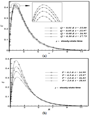 | Figure 5. The simulated steady-state velocity profile at X = 1.0 for (a) variation of Q with fixed P = 0.5; (b) variation of P with fixed Q = 0.05 |
4.2. Temperature
- The simulated transient temperature (T) for different values of Q and P with respect to t is shown at the point (1, 1.09)
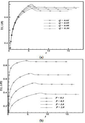 | Figure 6. The simulated transient temperature at (1, 1.09) for (a) variation of Q with fixed P = 0.5; (b) variation of P with fixed Q = 0.05 |
 and promotes greater surface temperature variations as shown in Fig. 6b.
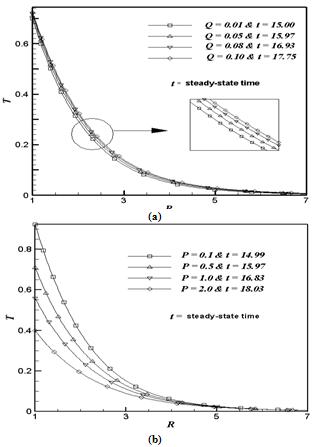 | Figure 7. The simulated steady-state temperature profile at X = 1.0 for (a) variation of Q with fixed P = 0.5; (b) variation of P with fixed Q = 0.05 |
 or higher convective cooling effect due to greater
  increases the value of P as well as causes greater temperature difference between the two surfaces of the cylinder. This is due to the reason that the temperature at the solid-fluid interface is reduced since the temperature at the inner surface of the cylinder is kept constant. As a result the temperature profile as well as the velocity profile shifts downwards in the fluid. It is also observed that the time required to reach the steady-state increases as P increases.
4.3. Average Skin-friction Coefficient and Heat Transfer Rate
- For engineering purposes, one is usually interested in the values of the skin-friction coefficient and heat transfer rate. The friction coefficient is an important parameter in the heat transfer studies since it is directly related to the heat transfer coefficient. The increased skin-friction is generally a disadvantage in technical applications, while the increased heat transfer can be exploited in some applications such as heat exchangers, but should be avoided in others such as gas turbine applications, for instance. For the present problem these skin-friction coefficient and heat transfer rate are derived and given in the following equations:The wall shear stress at the wall can be expressed as
 | (18) |
 | (19) |
 to be the characteristic shear stress, then the local skin-friction coefficient can be written as
 | (20) |
 | (21) |
 | (22) |
 is given byThus, with the non-dimensional quantities introduced in Eq. (10), Eq. (22) can be written as
 | (23) |
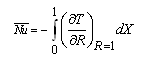 | (24) |
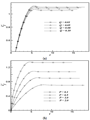 | Figure 8. The simulated average skin-friction for (a) variation of Q with fixed P = 0.5; (b) variation of P with fixed Q = 0.05 |
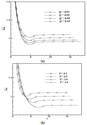 | Figure 9. The simulated average Nusselt number for (a) variation of Q with fixed P = 0.5; (b) variation of P with fixed Q = 0.05 |
5. Conclusions
- A numerical study has been carried out for the conjugate heat transfer on unsteady natural convection boundary layer flow of a viscous incompressible fluid over a vertical slender hollow cylinder with heat generation effect. A Crank-Nicolson type of implicit method is used to solve the governing unsteady, non-linear and coupled equations. The resulting system of equations is solved by using the Thomas algorithm. The computations are carried out for different values of heat generation parameter Q ( = 0.01, 0.05, 0.08 and 0.10) and conjugate-conduction parameter P ( = 0.1, 0.5, 1.0 and 2.0). For the velocity and temperature profiles it is observed that the time elapsed to reach the temporal maximum increases with the increasing values of Q and P. Time required to reach the steady-state increases as Q or P increases. It is observed that the velocity, temperature and average skin-friction coefficient of the fluid increases with the increasing values of Q. The values of velocity and temperature of the fluid decreases as P increases. It is also noticed that as P or Q increases the steady-state values of average heat transfer rate decreases.
ACKNOWLEDGEMENTS
- The authors wish to acknowledge support for this research work from the Institute Fellowship (National Institute of Technology Warangal).