1. Introduction

In the development of cancer, it has been shown that the exposure to hypoxia either induces or selects for cells that are hyperglycolytic, a reduction in cellular metabolism, and this in turn produces local acidosis which is a common feature of solid tumors[21,35,22]. Increased glucose uptake in hyperglycolyzing tumor cells is the basis of lesion-visualization in positron emission tomography using 18F-fluorodeoxyglu- cose[23,21,35]. Tumor acidity has been shown to reduce the effectiveness of weak-base drugs, therefore, by increasing the anti-tumor activity of weak-acid chemotherapeutics can serve as a biomarker for drugs effectiveness[34]. Physical removal, Chemotherapy and recently, adoptive immunotherapy have been sight-lined as methods used for attacking and managing cancer at various stages in their development[37,19]. However, some chemotherapeutic agents have been shown to increase the acidic content of the tissue and also causing mutations to non-tumor cells[36,7,20,9]. Evidence linking tumor acidity with increased activity of several extracellular matrix-degrading enzyme systems has been examined[23,11]. High levels of lactate which is an end-product of glycolysis, in primary lesions have been correlated with increased likelihood of metastasis[34]. It is therefore a complex story trying to administer chemothera-peutic drugs to treat this disease since it may accelerate the death of patients in particular if the therapy increases the acid production. In particular, it has been shown that when chemotherapy is administered, a toxic drug is introduced that in principles destroys all types of cells to some extent[6]. A thorough understanding of this tumor as it develops into cancer is required for administering chemotherapy and other therapeutics[16,17]. As we have seen, a guide to the understanding of this complex multidisciplinary concept is the fractional reaction diffusion model for cancer already discussed in[33]. The development of a cancerous tumor is a complex process involving the interaction of many types of cells[8,14,37,20]. The tumor itself is non homogenous and normal tissue, lymphocytes, macrophages and other types of cells either grow at the tumor site or are recruited to the tumor through chemotaxis[24,3,34]. Through biochemical process, all the cells involved in the metastases of tumor will interact. For example, immune-genic tumor cells and cytotoxic immune cells interact first binding to form cell conjugates, and then splitting to produce lysed tumor cells, inactivated immune cells, undamaged tumor cells or undamaged immune cells and debris[26,25]. The immune cells are responsible for the body immune system[16]. This immune system is a remarkable adaptive defense system that has evolved in vertebrates to protect them from invading pathogenic microorganisms and cancer. It is able to generate an enormous variety of cells and molecules capable of specifically recognizing and eliminating an apparently limitless variety of foreign invaders[16,26]. The combined action of these immune cells is referred to as immunity.

Mathematical models for immune interaction provides an analytic framework in addressing specific question about tumor-immune dynamics. Many such models have been studied and applied to clinical observations (also see ref. [6,8-11,13,15]. Since the fractional reaction diffusion model predicts the situation of death coming faster, a model incorporating immunotherapy, chemotherapy and feeding habit will show the way all these parameters will interact so as to predict the way drugs and food can reduce the death rate or increase the lifespan of the patient.

2. Model Consideration

We now modify the model of Oyesanya and Atabong[33] and Atabong and Oyesanya[1,2] to take cognizance of the effect of immunity and chemotherapy. In doing so, we note the following considerations;

• Drugs intake contribute a fraction to the total intake of a cancer patient given by .

• A constant dose of drugs taken at particular time and given by

• Acid removal nutrients contribute a fraction to the intake given by and a constant amount is taken periodically given by

• Chemotherapy also contribute a fraction of the intake given by and the quantity taken at any time t is given by, .

• Let be the total intake of drugs, chemotherapy and food such that, with the negative sign indicating that the intake are absorbed with time.

• The intake helps to recruit normal killer cells and activate CD8+T cells by a fraction given according to de Pillis et al. as where M is the tumor cell population and g and h are parameters included by De Pillis et al. to fit their model.

• The intake will also help to destroy tumor cells by a fraction given according to de Pillis et al. as where M is the tumor cell population and s and are parameters included by De Pillis et al. (2003a). to fit their model. The parameters and are the killer and recruiting terms respectively. Therefore the tumor and normal cells need not be the same since the properties of the tumor and normal cells are different.

• The intake H will result in killing of normal cells by a fraction given by where is a saturation term indicating the rate of absorption of H and is the dying rate.

• In the process of eating various kinds of food, some of them promote the development of tumor by a quantity given by. Where L is the acid production. The inverse proportionality to the population of the normal cells is because as the normal cells increase, the volume under consideration increase thereby reducing the pressure in the region and consequently the effect of the food substance is reduced according to Boys’ law as related to solids and liquids.

• Some of the tumor cells will be directly eaten up by chemotherapeutic agent and is given by, .

• The acid secretion shall be boosted by a proportion of the food taken and is given by, .

• Acid production will equally be inhibited by drugs at a rate

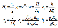
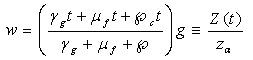
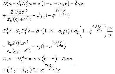
These assumptions combined with the original assumptions of Oyesanya and Atabong[33] coupled with the law of conservation of matter in a fixed volume of random movement, gives the non-dimensional modified fractional reaction diffusion model equation as;

Where the non-dimensional quantities are defined by

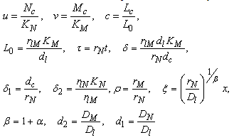(4.6)

And D_MN and D_NM are assumed to be relative and logistic since when the tumor has reached a certain size, the blood vessels are blocked by the growth, and the tumor cannot extend further. The normal cells on their part cannot exceed their growth capacity of the region when surrounded by the tumor cells. We defined the terms as shown in equation (5) below with the terms and being the constant diffusion coefficients of the Acid and the drug/nutrient;

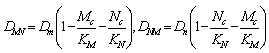(4.5)

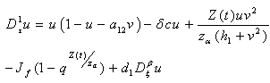
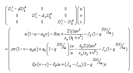
Substituting equation (4.6) into the system of equations (4.1,4.2,4.3,4.4) and using the simplified notation, , leads to the non-dimensional equations,

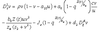
(4.7)

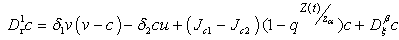
(4.8)

(4.9)

(4.10)

From these non-dimensional equations, we obtain the steady state constant solution by setting the spatial and temporal derivatives to zero. The equilibrium intake is given by,

(4.11)

which if substituted into equations (4.7,4.8 and 4.9) gives,

(4.12)

(4.13)

(4.14)

These equations therefore give us the interaction between the normal, tumor and acid secretion in the tumor region. These equations could be written as,

(4.15)

.

The equation (15) could further be written in matrix form as,

(4.16)

Suppose we set, then we may write the system (4.16) as,

(4.17)

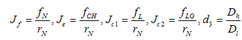
where the column vector and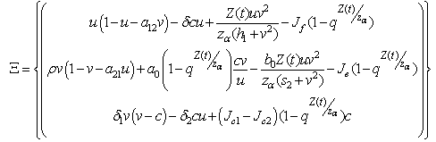

We define the following functions;

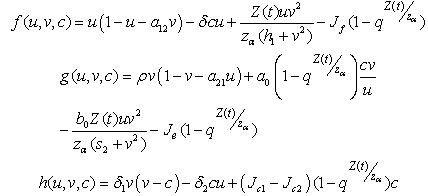A proper study of (4.17), will give us an understanding of the effect of the different parameters considered for the system. To start with, we obtain the steady state from, the kernel of .

i.e

Theorem 2: The disease free steady state exists and also if the patient does not die, then the patient will live without tumor (i.e. the steady state where u is not zero and v is zero exist and such a state is realistic and u will have a maximum value if

Proof

It is clear that, if there are no normal cells then there will be no tumor cells and in this case, the disease-free state will exist but the patient is not living. Hence it suffices to show that if , then u is maximum which in non dimensional scale parameters is unity.

If v=0 in (4.19) and we have, and whenever, , we get that .

Claim1: Suppose we define a function 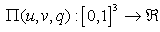such that,

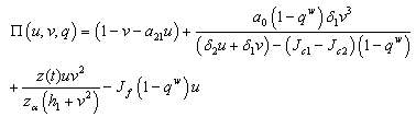If in addition we supposed that 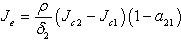when ever and =0, then either, the quantity or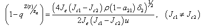

Proof (Claim)

From equation (4.20),

This is a quadratic in and from this equation, we get that,

Solving we get,

, where are the coefficients of the quadratic middle and constant terms respectively and are defined as follows;

Clearly, the claim follows by substitution.

Remark 1

Since can either be increasing or decreasing, we consider the case where, . In this case, we must have that,

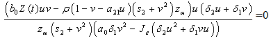if and then,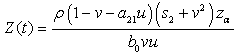

by simplification.

Therefore this is the value of the intake to sustain the patient. We consider 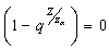in this work as a situation where the drugs are prescribed, taken by the patient regularly as and the body system is reactive to the drug by absorbing it at a proportional rate.

Theorem 4: If the prescriptions of food and drugs are followed strictly (taken at the right time and right dose), and if in addition then the only realistic steady state is the disease free steady state.

We consider a regular timely therapeutics intake to be a case where the constant intake Z(t) at any time is 1.

That is,

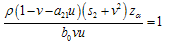Multiplying this expression out when u=1 gives,

from where we get,

which could simplify to,

(4.21)

From considerations of the cubic equation, suppose then equation (4.21) by the Descartes rule, has no positive root and the only realistic value for v in this case which could be obtained when Hence we conclude that the disease-free state is the only possible state.

3. Stability of the Disease-free Steady State

We now study the stability properties of the disease-free steady state using the following theorem.

Theorem 5: If the therapeutics are absorbed on time regularly on time i.e. the disease free state is stable for 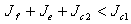, and if the therapeutics are not regularly absorbed and on time i.e. , then the disease free steady state is stable for .

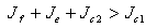Proof

Linearizing equations (4.7,4.8 and 4.9) about the disease-free steady state gives,

(4.22)

where

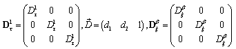
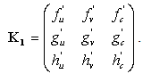A solution in exponential form gives a Jacobian of the form,

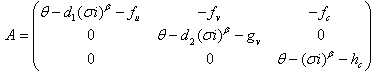where,

.

We obtain a dispersion relation from the equation

(4.23)

from where we get,

(4.24)

Hence, and

(4.25)

The roots of equation (4.25) are complex therefore we need to determine the real and the imaginary parts of these roots to determine stability of the system (Beck et al., 2009).

The roots of (4.25) are given by,

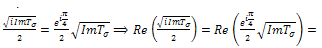
Remark 2

If ₵ such that z=a+ib with then .

We make the substitution,

We make the following representations,

where

(4.26)

From remark 4.2 we see that will be of the form a+ib.

We now determine the sign of by considering the expression (4.26) and write,

(4.26a)

which we can write as

(4.26b)

We look at different cases of the expression in (4.26b) for namely,

Case 1: =0 and

In this case, equation (4.26b) becomes,

Since . Therefore, the sign of depends on the sign of 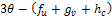and the sign of. In addition, if then, sign of depends only on the sign of and on substitution of the values of the first partials the expression will simplifies to

If for stability, 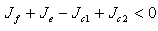provided the therapeutics are timely absorbed. This is equivalent to,

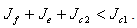On the other hand if the therapeutics are not timely absorbed, i.e. some accumulate for some time before absorption, then and in this situation, for the disease-free state to be stable we must have, which is equivalent to,

If , then for us to have stability, .

Suppose then the situation changes and we get,

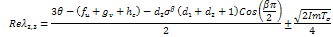Replacing by their values gives,

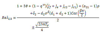Stability is therefore a function of the sign of whose sign depends also on both the signs of

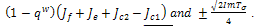. For the case where, for the first root, λ₂ and we make the following deductions;

If the sign of each of the two roots can be determined as follows. For the first root, the sign, will depend on the sign of which is required to be negative as a condition for us to get stability.

Hence,

For the second root, the sign of will depend on the sign of which is required to be negative as a condition to for us to obtain stability.

Hence,

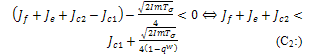Since both roots must have their real parts negative for stability, the two conditions (C₁:) and (C₂ ) implies, .

For the case where, will become, . The real part of the roots shall therefore be,

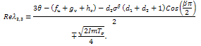The conditions for stability will not change since the only difference in this case is the replacement of the sign, with the sign, . The condition for stability on the first root will become that of the second root in this case while that of the second root will become the condition of the first root, both of which will lead to the unique condition,

.

Case 2: and

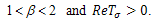In this case,

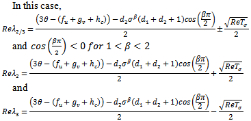Substituting the partials gives,

and the sign of this root will lead to these conditions as Case (1) above.

For the third root we must have,

Case3: and

In this case, a situation of hopf bifurcation is possible if one of the following conditions is true; or and.

A necessary but not sufficient condition for this to occur is,

and

This way we have established that the disease-free equilibrium is stable for and can also bifurcate if in addition to this condition, we have other conditions like those stated in case3. This therefore ends the proof of theorem 4.5.

In proving the stability of the disease free state we have looked at the main case where . We now throw light in the case where in order to know if the conditions will change.

We now consider the case of our fractional variable, is such that, .

In this case, the real parts of the roots,

will not only depend of the sign of but on the sign of,

as a whole.

If we make our usual substitution in the first case,

We get,

If the therapeutic intake is absent, then.

Since, , if then stability will depend of the sign of

With respect to the first root,

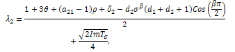We must have that,

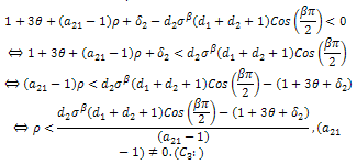With respect to the second root,

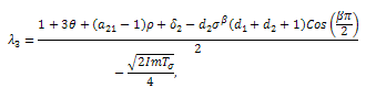We must have that,

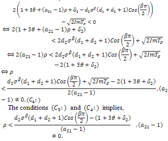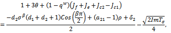
On the other hand, in the presence of therapeutics i.e. keeping away the condition, by setting, we get as the real part of the roots and the expression,

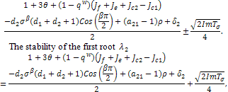mostly depends of the sign of,

, since all the other terms are positive.

Hence,

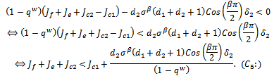The stability of the first root

mostly depends of the sign of,

since all the other terms are positive.

Hence,

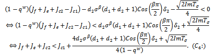The

conditions and implies,

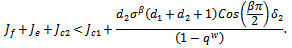
is inferior to all other conditions for stability if the therapeutics are regularly absorbed. In this light, we concluded that;

If the therapeutics are not absorbed at all (i.e. ), then for the disease to be eradicated,

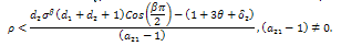If the therapeutics are absorbed irregularly and inconsistently, then for the disease to be eradicated,

If the therapeutics are absorbed irregularly and consistently, then for the disease to be eradicated,

We have therefore shown the different conditions for the disease to be eradicated or for it to persist and possibly leading to death of the patient. In the next section we look at the numerical simulation of the full nonlinear fractional reaction diffusion equation by discretization.

4. Numerical Simulations

In this section, we apply numerical method to solve the system of fractional reaction diffusion equation. In the literature, most numerical methods of fractional reaction diffusion equation were done for single equations and not for a system of equations. However, we shall apply some of the established results for single equation in order to obtain a corresponding numerical method for systems. The idea is to know how the drugs and other therapeutics will affect the growth rate of the tumor cells as well as normal cells.

To study the behavior of the tumor cells, we simulate the entire system for different boundary conditions.

We will apply the same process to get an equivalent central difference formula for the fractional diffusion equation.

Since the fractional order is relative to space, we obtain a discretized -order fractional derivative using the Grunwald finite difference formula[32]. Also see the literature such as[18,27,28,31] for more insight into finite difference fractional reaction diffusion equation. We used the second order accurate finite difference formula for the fractional diffusion equation which has been established Tadjeran and colleague in 2006, namely,

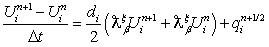(4.29)

where,

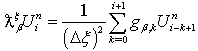and are the Grunwald weights.

Applying these estimates into our system of fractional reaction diffusion equations through a program which solves the system by applying Gauss elimination process using the algorithm presented in appendix C we have the results depicted in the figures in appendix B-3.

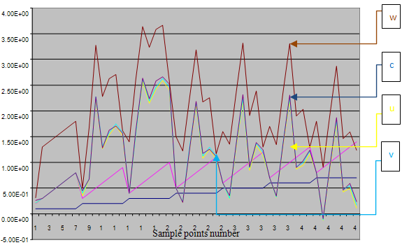
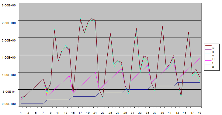
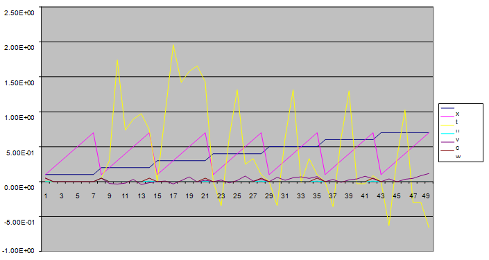
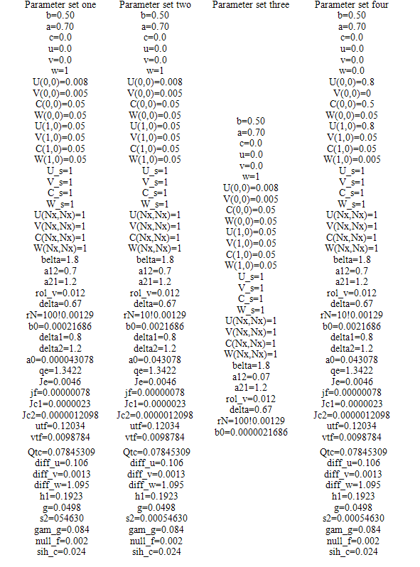
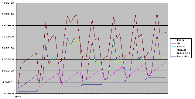
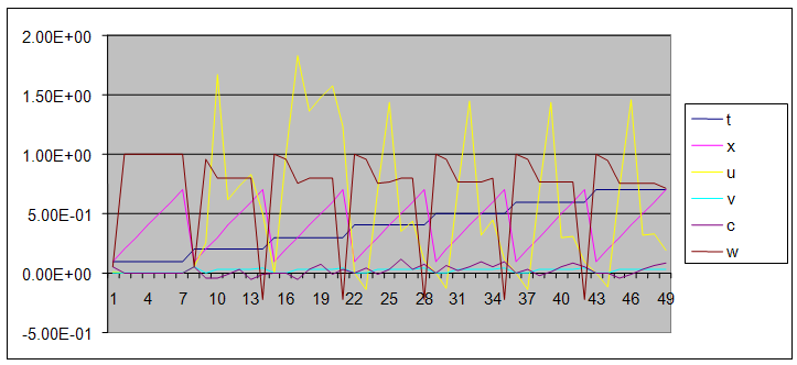
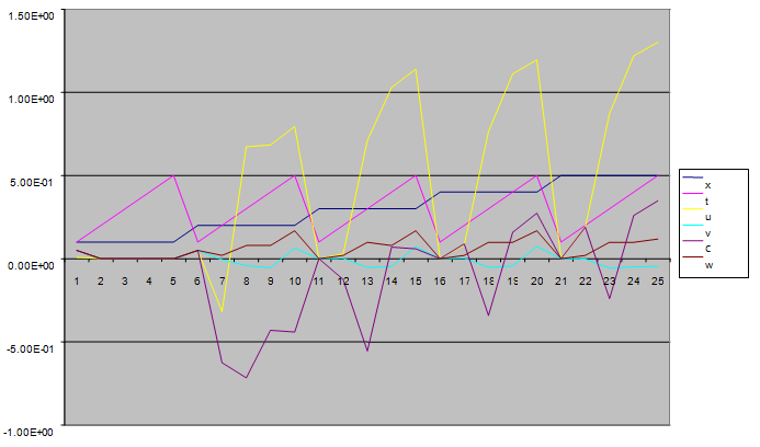
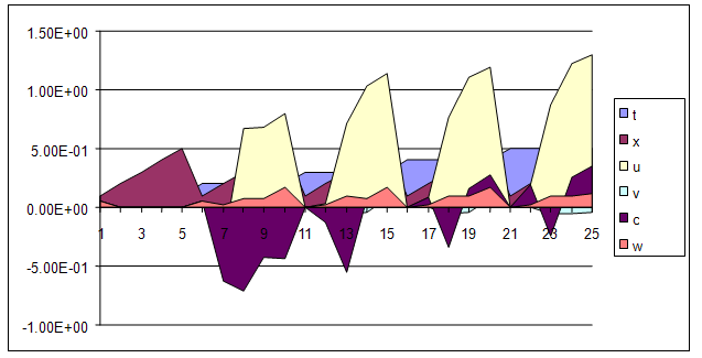
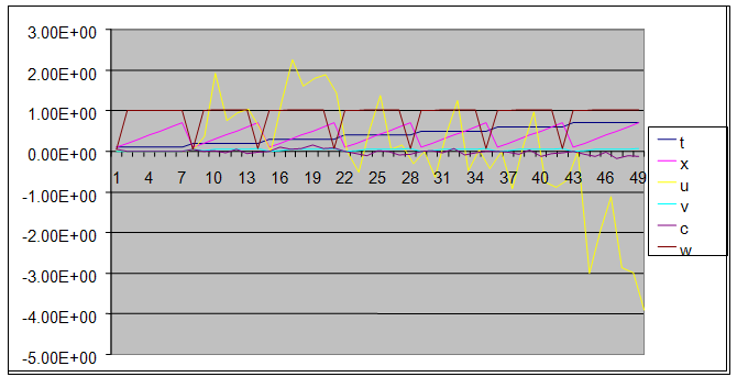
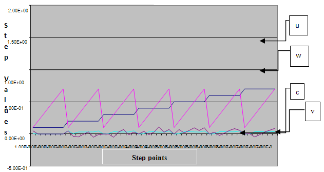Figure 1. A free line plot of Normal, Tumor, H+ Concentration and Therapeutic intervention as against time and space with parameter set one

Figure 2. A free line plot of Normal, Tumor, H+ Concentration and Therapeutic intervention as against time and space with parameter set one

Figure 3. :A free line plot of Normal, Tumor, H+ Concentration and Therapeutic intervention as against time and space with parameter set one

Figure 4. A free line plot of Normal, Tumor, H+ Concentration and Therapeutic intervention as against time and space with parameter set one

Figure 5. A free line plot of Normal, Tumor, H+ Concentration and Therapeutic intervention as against time and space with parameter set one

Figure 6. A free line plot of Normal, Tumor, H+ Concentration and Therapeutic intervention as against time and space with parameter set one

Figure 7. A free line plot of Normal, Tumor, H+ Concentration and Therapeutic intervention as against time and space with parameter set one

Table 4.3. Table of different parameter sets for numerical simulation of therapeutic reactions

Figure 8. A free line plot of Normal, Tumor, H+ Concentration and Therapeutic intervention as against time and space with parameter set one

Figure 9. A free line plot of Normal, Tumor, H+ Concentration and Therapeutic intervention as against time and space with parameter set two

Figure 10. A free line plot of Normal, Tumor, H+ Concentration and Therapeutic intervention as against time and space with parameter set two

Figure 11. A free line plot of Normal, Tumor, H+ Concentration and Therapeutic intervention as against time and space with parameter set two

Figure 12. A free line plot of Normal, Tumor, H+ Concentration and Therapeutic intervention as against time and space with parameter set three

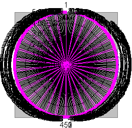Figure 13. A chart showing the diffusion pattern of all four spaceis in the absence of reaction and production terms

5. Results and Discussion

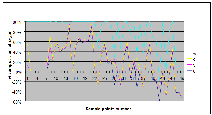
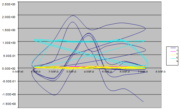
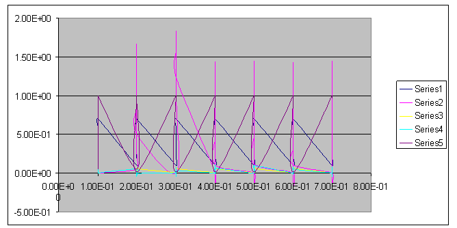
We present a discussion of the figures in the following paragraphs in a chronological order.

Figure 1 shows a situation where the therapeutics has clearly controlled the growth of tumor cells leading to a comfortable increasing growth of normal cells. This was obtained by increasing the value of per-capita normal cell growth r _N this goes to reduce the rate of therapeutic absorption and therapeutic intake. In this case, the tumor cells emerge in the organ and at once some of the therapeutic actions accelerate the production of more immune cells which led to the broad increase of normal cells in the region at the second time step. This increase is advanced to a maximum at the third time step and the tumor cells are eradicated at this stage but resurface again at some point in the region at the same time step. An increase in concentration of H+ is immediately seen at this region which leads to a slight reduction in the concentration of normal cells. From this point upward, the normal cells attain a constant amplitude and as the number of time step is increased the number of tumor cells is fluctuating in the neighborhood of zero. This shows that the application of therapeutic can eradicate the tumor; however, in the case where the tumor reappears, maintaining the constant value of therapeutic intake will not eradicate the tumor since reappearance of the tumor can be seen as a situation where the tumor has become resistant to the therapeutic intake.

Figure 2 shows a situation where all therapeutics are suppressed in order to get a caricature of the model in Oyesanya and Atabong[33]. The model shows that the population of tumor cells is always above the population of the normal cells in the region (organ) of attack and the death situation appears in a finite time step. In this case, the tumor emerged and grows periodically, eating up the normal cells. The concentration of H+ also increases proportionally at the detriment of the normal cells resulting to the destruction of more normal cells. This was also seen for different parameter values in[33]. However, there the functions were evaluated in real and imaginary part separately in a numerical integration while in the functions are evaluated in couple in these simulations in general and the simulation presented in figure 4.6 in particular.

Figure 3 is a complicated situation where all three species are competing and leaving in the patient. In achieving this figure, we consider the value of J_c1 to be greater than the sum of the values of the fractional therapeutic intakes, J_e, J_f and J_c2. As the tumor cells increase, the therapeutics increase and boost the production of more normal immune cells. As a result, the tumor cells are reduced by the inhibiting actions of the normal immune cells. This is however not stable since the effect of this reduction felt by the immune system which immediately reduces the value of the therapeutics absorbed since more immune cells are activated to fight against defense. The tendency here is that the tumor will pick-up again and the process will continue.

Figure 4 shows the situation where the value of J_c1 was made to be less than the sum of J_e, J_f and J_c2. The disease-free state appears after some finite time step and is stable. The tumor is under control but however, it still resurface at every time step if the level of therapeutics is zero. This shows that once therapeutic strategies comprising chemotherapy and immunotherapy is applied for the treatment of cancer, the food intake for which the patient is prescribed to take must be continued even after the cancer is eradicated. Neglecting the treatment will lead to a re-invasion of the cancer which may become more dangerous.

Figure 5 shows proportional plot for contributing species in the region of attack. Each of the population is compared to the total proportion of the species in the region already existing. In other words, the population of tumor, normal cells, acid and therapeutics in the proliferation region within the parameter domain of parameter set one is compared to each of these species in turn. The proportions of tumor cells are continuously above that of the normal cells. The death situation will therefore arise after some time step as the figure shows.

Figure 6 shows a pattern plot of the four interacting species in which we see that the normal cells and the therapeutics display more complex pattern than the tumor and H+. It rightly indicates a situation where the tumor will be eradicated. The parameters considered here are shown in table 4.3 appendix A under parameter set 1.

Figure 7 shows a plot which is connecting all the interacting species with respect to time. As can be seen from the figure, the normal cells are dominant over the tumor cells which are consequently eradicated at the six time step. The parameter set two as shown in table 4.3, appendix A was considered for this simulation.

Figure 8 is a simulation with a full set of different parameters as shown in parameter set one, table 4.3 in the appendix A. Worth noting, is the significant reduction of b₀ a consequence of an increase in g or reduction in g₂ which are parameters for model fitting as shown in[13,15] and a significant increase in the value of s₂ (also for fitting the model by De Pillis and Radunskaya in[9-11]) to a value of 054630. The value of the normal cell per capital birth rate is also increase to 100 cells per unit time. The plots show a periodic variation in which the normal cells population is always below the tumor cells population. The figure does not show if one of the species eventually dies but based on our analysis, such a state is not stable and can always turn in favour of any one of the species at any time.

In figure 9., the values of b₀, s₂ and a₀ and r_N were taken to be, r_N=10, b0=0.0021686, a₀=0.43078 and s₂=0.00054630. Increasing a₀ is as a result of the reduction of r_N. The plots shows that the normal cells are comfortable in the region at the detriment of the tumor cells. The concentration of acid in this region is reduced and maintained constantly by the therapeutic intake. This is however, proportional to the invisible proportion of the tumor cells as shown in the simulation.

A slight increase in r_N, while maintaining the value of b₀ and a₀, leads to an increase in the absorption of acid and a clear situation of the eradication of the tumor is seen as shown in figure 10. A two dimensional plot of the simulation result is shown in figure 10 for a clearer view.

In figure 11, the parameter set three of table 4.3 in appendix A is considered with some minor changes key variables. In this parameter set, the values of b₀ and a₁₂ are reduced to 0.0000021686 and 0.07 respectively. The plots shows that the normal cells quickly drops below the tumor cells and consequently the death of the patient is seen as all values of the normal cells are negative.

Figures 12 is a simulation of the system with parameter set 4 as shown in table 4.3 of appendix A. In these plots there is no normal cell showing that the tumor is diagnosed only after it had affected all basic organs of the patient. The tumor grows in the region uncontrollably in the acid secretion. This shows that the therapeutics accelerates the death of the patient in this case. This confirms the fact that some therapeutics helps in killing normal cells.

Figure 13 is a simulation without the interaction of the species in this case, the function values were considered to be zero. The results show nothing different from the solution of the fractional heat equation and can therefore be used as a numerical result of the fractional heat equation.