K. V. Zhukovsky 1, G. Dattoli 2
1Faculty of Physics, Moscow State University, Leninskie Gory, Moscow, 119899, Russia
2ENEA Research Centre, Fis-Mat, 00044, Frascati, Rome, Italy
Correspondence to: K. V. Zhukovsky , Faculty of Physics, Moscow State University, Leninskie Gory, Moscow, 119899, Russia.
| Email: |  |
Copyright © 2012 Scientific & Academic Publishing. All Rights Reserved.
Abstract
We analyse and demonstrate how umbral methods can be applied for the study of the problems, involving combinatorial calculus and harmonic numbers. We demonstrate their efficiency and we find the general procedure to frame new and existent identities within a unified framework, amenable of further generalizations.
Keywords:
Umbral, Identities, Calculus, Harmonic Numbers
Cite this paper:
K. V. Zhukovsky , G. Dattoli , "Umbral Methods, Combinatorial Identities and Harmonic Numbers", Applied Mathematics, Vol. 1 No. 1, 2011, pp. 46-49. doi: 10.5923/j.am.20110101.06.
1. Introduction
In this article we employ methods of umbral nature to provide a common framework for known and new identities regarding combinatorial calculus and harmonic numbers. Just to give a glimpse into the technique, adopted in this article, we remind the identity [1]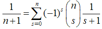 | (1) |
which, after defining the umbral variable  (see[2]), where 1 — the vacuum state of the space, on which the operator
  acts, and
 — the unit operator:
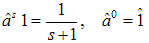 | (2) |
can be cast in the following form: 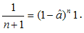 | (3) |
Equation (1) can be written in the form (3) just as the consequence of the binomial theorem and of definition (2) and it is a useful tool to generate new identities, listed below:a) The duplication “theorem”: 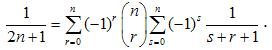 | (4) |
The proof of this last identity is easily achieved by following the steps outlined below. We can obtain the obvious consequence of the equation (3):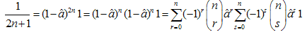 | (5) |
thus getting equation (4) from the identity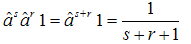 | (6) |
b) The “addition” theorem: 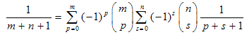 | (7) |
c) The multiplication theorem: 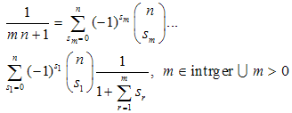 | (8) |
The proof of b) and c) theorems is achieved by the same procedure leading to the proof of a) and is omitted here for the sake of conciseness1 Now let us introduce the operator of the umbral derivative, defined by the following rule: 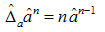 | (9) |
which, along with the multiplication condition: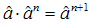 | (10) |
yields the following result for the commutator bracket between the two operators: 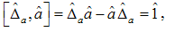 | (11) |
Equation (11) ensures that, we can benefit from the properties of the Weyl-Heisenberg algebra, characterising our problem. Within this framework the following simple example is provided by the definition of the associated Hermite polynomials: two variables Hermite polynomials are defined below with the variable x replacing the operator  as follows2:
 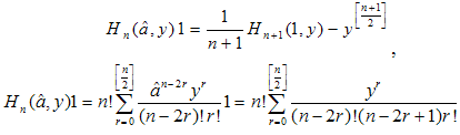 | (12) |
It is easy to show that the following recurrences are satisfied: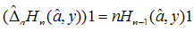 | (13) |
and 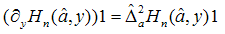 | (14) |
which are direct generalisations of the relevant to the ordinary Hermite polynomials relations. The umbral heat equation (14) can be exploited to define the polynomials (12) in terms of the following operational equation: 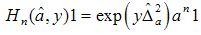 | (15) |
In these introductory remarks we have presented few elements of the formalism, which we employ in the following chapters to further develop the method of umbral operators and obtain new identities in combinatorial calculus, involving the Euler Beta and Riemann Zeta functions.
2. Umbral Methods and the Euler Beta Function
Let us take note that the parameter n in the equation (1) can be treated as a variable and, therefore, p times repeated derivatives with respect to n can be taken on both sides: 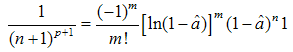 | (16) |
Now, using the following series expansion [4]: 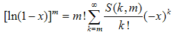 | (17) |
assumed to be valid also for the umbral operator , we end up with the following identity:
 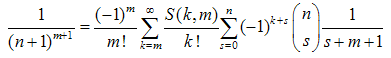 | (18) |
where  — the Stirling numbers of the first kind [4]. The validity of (18) has been checked aposteriori by a numerical procedure. Explicit study of the Stirling numbers relations with combinatorial identities can be found in[5]. Note, that identity (18) involves infinite sums and they can be avoided, if we rewrite (18) with the help of the identity
 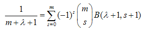 | (19) |
where  — the Euler Beta function, which writes in terms of the Euler Gamma function as follows[6]:
 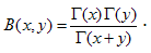 | (20) |
We proceed on the assumption that the above definition (20) is valid also for the umbral variable  to write (19) in the following form:
 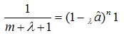 | (21) |
where we denoted the power of the umbral variable  via the beta function as follows:
 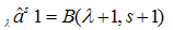 | (22) |
Therefore, we can reformulate all the theorems a) – c) in a fairly direct way in terms of Beta function. For example, the duplication identity can be written as follows: 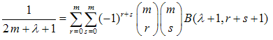 | (23) |
Taking repeated derivatives of both sides of (19) with respect to λ in the point λ = 0 yields the r power of the left-hand side of equation (18), written in terms of the Beta function instead of the Stirling numbers: 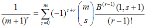 | (24) |
where 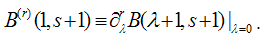 | (25) |
This last result (24) represents essentially the equation (18), written without any explicit use of infinite sums. As to the explicit evaluation of the derivatives of the Beta function, we note that they possess the integral representation, provided by[6,7]: 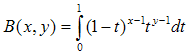 | (26) |
and, therefore, we find the following expression for the derivative of the Beta function: 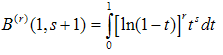 | (27) |
In the next chapter we will apply the above obtained results to the theory of the harmonic numbers.
3. Umbral Methods and Harmonic Numbers
The harmonic numbers[8] are usually denoted by Hn; to avoid confusions with Hermite polynomials we use here hn notation: 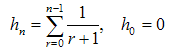 | (28) |
Umbral methods technique simplifies the derivation of the properties of the harmonic numbers and the study of the associated generating functions. We can express the harmonic numbers (28) in terms of the umbral variable (2) as follows: 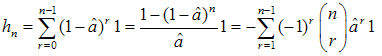 | (29) |
and derive the following relation between the harmonic numbers and the umbral variable: 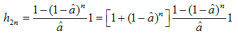 | (30) |
which eventually yields: 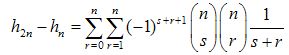 | (31) |
Further extensions can be easily obtained without conceptual difficulties, except for some cumbersome algebraic steps, for example: 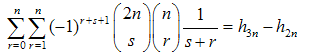 | (32) |
Analogous relations can be obtained for the generalized harmonic numbers, defined as follows: 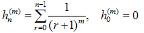 | (33) |
The use of the above described procedure and of the identities derived in the previous chapter 2 yields the generalization of the formula (32): 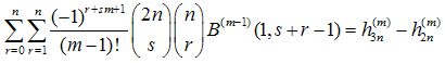 | (34) |
Further comments on umbral methods and harmonic numbers are given in the following concluding chapter.
4. Generalisations and Discussion
To complete the study of the harmonic numbers and umbral methods, consider the following sum: 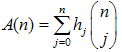 | (35) |
Employing the results of the previous chapter 3 we recast A(n) in the following operator form: 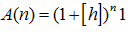 | (36) |
where operator [h] acts on the harmonic number hn as a kind of a raising operator: 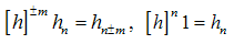 | (37) |
Recalling the generating function3, associated with the harmonic numbers[9]: 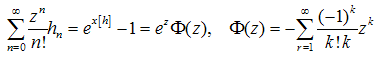 | (38) |
we write: 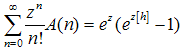 | (39) |
which, together with the obvious relation lead to the following identity:
 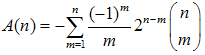 | (40) |
The generalization of the identity (40) lets us formulate the following theorems:a) The duplication theorem: 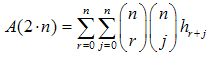 | (41) |
b) The multiplication theorem: 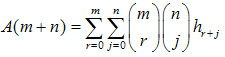 | (42) |
We can also define the higher order moment: 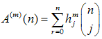 | (43) |
and associated with them function A(n, y): 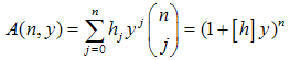 | (44) |
Then from the definition of the higher moment we obtain: 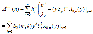 | (45) |
where — the Stirling numbers of the second kind. The
  can be obtained via the same procedure, which yielded (40), namely:
 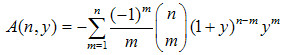 | (46) |
Eventually we obtain the high order moments 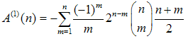 | (47) |
and 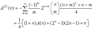 | (48) |
Higher than 2d order moments can be derived using the Stirling numbers and other new identities can be generated with the help of the Matematica software.In conclusion we would like to underline that the umbral methods we have exploited in this paper are strongly reminiscent of other methods adopted in literature to define e. g. the Bernoulli[4] or the Laguerre[10] polynomials. Consider the following polynomial family: 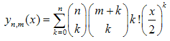 | (49) |
which reduces to the Bessel polynomials, introduced by Krall and Frinck in[11] for m = n. These polynomials can be defined in umbral terms as follows: 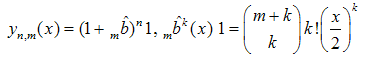 | (50) |
and they can be exploited to establish, for example, duplication or addition theorems or for other purposes. With the help of the identity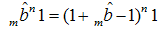 | (51) |
we can derive the following expansion of  in terms of the polynomials (50):
 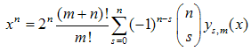 | (52) |
The umbral procedure applications, demonstrated in this work in respect of the harmonic numbers, can be useful also for the study of the relationship between different from each other families of polynomials. In forthcoming publications we will discuss it. In the context of the link between Bernoulli and Faulhaber polynomials[12,13] and we will apply the umbral procedure to solve some non-linear partial differential equations.
Notes
1. Also note that with the help of the identity  we further find the following relation
 .2. Multiplication condition (10) does not define any new polynomial family3. Eq. (38) is referred in literature as the Gosper Formula and it was derived in[9], whereas its generalisations were derived in [7], using umbral methods.
References
| [1] | L. Comtet, Advanced Combinatorics: The Art of Finite and Infinite Expansions, rev. enl. ed. Dordrecht, Netherlands: Reidel, 1974 |
| [2] | S. Roman, The Umbral Calculus. New York: Academic Press, 1984 |
| [3] | C. Hermite, "Sur un nouveau développement en série de fonctions." Compt. Rend. Acad. Sci. Paris 58, 93-100 and 266-273, 1864. Reprinted in Hermite, C. Oeuvres complètes, tome 2. Paris, pp. 293-308, 1908 |
| [4] | M. Abramowitz. and I. A. Stegun (Eds.). "Stirling Numbers of the First Kind." §24.1.3 in Handbook of Mathematical Functions with Formulas, Graphs, and Mathematical Tables, 9th printing. New York: Dover, 1972 |
| [5] | G. Dattoli, M. Migliorati, K. Zhukovsky “Summation Formulae and Stirling Numbers” Int. Math. Forum, 4, 2009, N41, 2017-2040 |
| [6] | L. C. Andrews, Special functions for Engineers and Applied Mathematicians New York: Mc Millan, 1985 |
| [7] | G. Dattoli, H.M.Srivastava, K. Zhukovsky. “Operational methods and Differential Equations with Applications to Initial-Value problems” App. Math. Comp.184, 2007, 979-1001 |
| [8] | Sondow, Jonathan and Weisstein, Eric W, Harmonic Number. From MathWorld — A Wolfram Web Resource http://mathworld.wolfram.com/HarmonicNumber.html |
| [9] | R. W. Gosper ”Harmonic Summation and exponential gfs.” math-fun@cs.arizona.edu posting, Aug. 2, 1996. (as reported in[8]) |
| [10] | G. Dattoli, H. M. Srivastava and K. Zhukovsky, “Orthogonality properties of the Hermite and related polynomials” J. Comput. Appl. Math. 182, 2005, 165-172 |
| [11] | H.L. Krall and O. Fink ”A New Class of Orthogonal Polynomials: The Bessel Polynomials” Trans. Amer. Math. Soc. 65, 100, 1948 |
| [12] | Roman, S. "The Bessel Polynomials." §4.1.7 in The Umbral Calculus. New York: Academic Press, pp. 78-82, 1984 |
| [13] | E. Grosswald, Bessel Polynomials. New York: Springer-Verlag, 1978 |
 Abstract
 Reference
 Full-Text PDF
 Full-Text HTML