1. Introduction

In systems with hysteretic behavior, like piezoelectics, piezoceramics, magnetostrictives and shape memory alloys, the input-output relationship is a multi-branch nonlinearity for which branch-to-branch transitions occur after input exterma[1]. It means that the output value is a function not only of the current input, but also of the previous inputs and/or the initial value. Indeed, at any accessible point in the input-output diagram there are many curves that may rep-resent the future behavior of the system. Each of these curves depends on the sequence of past extermum values of the input[2]. Therefore, mathematical modeling as well as controller design of these systems is a complex and difficult task.

Since un-modeled hysteresis causes inaccuracy in trajectory tracking and decreases the performance of the control systems, an accurate modeling of hysteresis behavior for performance evaluation and identification as well as controller design is essentially needed[3]. Therefore, it is necessary to develop hysteresis models that not only identification of the model parameters, to adapt the model to the real hysteretic nonlinearity, can easily and precisely be per-formed but also are suitable for real time control and compensation system design.

A number of models have been proposed to capture the observed hysteretic characteristics of smart actuators, which could be classified into physics-based hysteresis models and phenomenological hysteresis models[4]. Physics-based models are generally come from the underlying physics of hysteresis and are combined with empirical factors to de-scribe the observed characteristics[5-7]. However, these models have limited range of applicability, as the physical basis of some of the hysteresis characteristics is not completely understood[8]. Furthermore, considerable effort is required in identifying and tuning the model parameters to accurately describe the hysteresis nonlinearity. Another major drawback of these physical models is that they are specific to a particular system, and this implies separate controller design techniques for each system[9].

Since the early 1970's, systematic mathematical analyses of the hysteresis as a general nonlinear behavior, from purely phenomenological viewpoint, have been carried out[10]. Phenomenological models are based on the phenomeno- logical nature and mathematically describe the observed phenomenon without necessarily providing physical insight into the problems. The most important phenomenological hysteresis models include operator based hysteresis models and differential equation-based hysteresis models[11]. Preisach model[2], Krasnosel’skii-Pokrovskii model[1], and Prandtl-Ishlinskii model[12] are some important operator- based hysteresis models while Duhem model, Bouc-Wen model and Jiles-Atherton model[13] are most widely used differential equation-based hysteresis models. Choosing a proper phenomenological model among the mentioned models is a task of crucial importance since the mathematical complexity of the identification and inversion problem depend directly on the phenomenological modeling method and strongly influences the practical use of the design concept[14]. Furthermore, the accuracy of the modeling method in characterizing system hysteretic behavior consequently affects the whole compensator design task. For example, Philips[15] compared the computation results from the Jiles-Atherton model and the Preisach model. It was found that the identification of the parameters in the Jiles-Atherton model requires less measurement while the Preisach model fits the hysteresis loop better.

Modeling the SMA actuators by each of the mentioned groups has their own advantages and disadvantages. Models of the first group are better suited to deal with the effects of complex multiaxial thermomechanical loading paths and cyclic effects of SMAs, due to the flexibility of introducing internal state variables in their formulation. However, these classical models usually give poor predictions to the minor loop hysteretic response[16]. Phenomenological models, on the other hand usually give excellent predictions of the minor loop behavior if the loading path does not change.

Among the phenomenological models, the Preisach model has found extensive application for modeling hysteresis in SMAs and other smart actuators[17-18,2]. In Preisach modeling technique, overall system with hysteresis behavior is modeled by weighted parallel connections of non-ideal relays termed as Preisach elementary operators. Output of these Preisach operators would be only +1 or –1 (zero in some models). Every elemental operator as a nonlinear operator consists of two parameters; upper and lower switching values of input respectively. Along with the set of Preisach operators is an arbitrary weight function, called the Preisach Density Function (PDF), which works as a local influence of each operator in overall hysteresis model.

The time continuity of an operator is important for physical considerations, while the parametric continuity is important for designing well-posed identification methodologies[19]. However, the kernel of the Preisach operator has no continuity in time space or in parameter space. In[20] Banks et.al, introduced the smoothed version of the Preisach operator. To construct the continuous preisach operator in time space, they first define a smoothed delayed operator, each of whose ascending and descending branches are continuous. This continuous Preisach model yields a continuous output hysteresis, even for measures that are not absolutely continuous with respect to Lebesgue measure. However, this operator was also not continuous in parametric space.

In order to have continuous operator in time domain as well as in parameter space Krasnosel’skii-Pokrovskii[12] allowed the Preisach kernels to be any reasonable functions. The KP type operator, a special case of a so-called generalized play operator, is a hysteretic operator treating continuous branches rather than jump discontinuities like in the Preisach operator. This kind of generalization finally separates the Preisach model from its physical meaning and ends up with a purely mathematical and phenomenological operator[21]. This generalized Preisach model has been further investigated and applied in[20], where kernels other than non-ideal relay operators are employed to achieve some mathematical properties. Banks et al.[20] proved that K-P operators are continuous in time as well as in parameter space. They also compared the physical and mathematical properties of K-P operator with those of the classical Preisach operator.

Since the original integral form of the KP model easily cannot numerically and practically implemented, the linearly parameterized KP model usually applied. This stems from these reasons that it is very difficult to formulate suitable weighting function which is double-integrable and also it is impossible to describe the outputs of the kernel as continuous functions due to nonlinearity of the kernel[22]. In this method, a finite number of the kernel functions is utilized and each kernel function itself stands for a reasonable approximation of actual hysteresis curves of the actuator.

There are many experimental researches about modeling SMA actuators by Preisach model in order for evaluating and predicting their behaviors but using the KP model in this area is much less. Webb et al.[23] presented an adaptive hysteresis model, which was a linearly parameterized version of the KP hysteresis model. This model can be updated continuously by using adaptive method so that it can describe the hysteresis behavior of an SMA wire actuator successfully under extended disturbances and various loading conditions. They provided laboratory evidence of the success of the proposed adaptive KP model for feedback control of an SMA wire actuator. Since the proposed KP hysteresis model can adaptively identify, it is robust in the presence of large measurement errors. Moreover, by computing the inverse of it, the effect of the hysteresis in SMA actuator can be actively compensated. Koh[24] used a similar adaptive control technique with a KP hysteresis operator. It was shown that the inverse of hysteresis behavior also has qualitatively the same characteristics of hysteresis. Therefore, in order to evade the computation of the inverse of the KP model, the inverse model with KP hysteresis operator was directly used. Finally, the result of the proposed controller is experimentally compared with ones of a PI controller.

In[25] Galinaitis demonstrated the ability of KP model to model hysteresis of piezoelectric actuator and also the effectiveness of the inverse compensation to minimize hysteresis. In addition using the experimental data collected from a piezoelectric actuator with scalar hysteresis, the accuracy of the forward model was also demonstrated. Furthermore, the feasibility of using inverse of KP model to provide the necessary compensation for reducing positioning error created by hysteresis was displayed.

In most of the researches conducted about the modeling of SMA actuators by KP model, only the ability of the KP model in characterizing the hysteretic behavior of the actuators is demonstrated with respect to some specified experimental data and the accuracy of the developed model with respect to other data is not validated. In other words only the parameters of KP model are identified in order to adapt the model response to the real hysteretic nonlinearity with some specific experimental data and finally the outputs of the obtained KP are compared with those same data. Therefore, it is not clear whether the developed model is capable in predicting hysteresis minor loops of SMA materials or not and how its accuracy in this prediction task is. Some of the shortcomings of the mentioned studies are due to the fact that the tested actuator was not available in the laboratory and therefore further experimental tests were not performable. Also, if the inverse of the KP model is a candidate for hysteresis nonlinearity compensation using an open loop feedforward controller, it is important to know how accurate the developed model would model the ob-served input-output relation and determine whether using a feedback controller is essential or not.

In this paper, first the parameterized KP model is identified by some experimentally measured data obtained from an experimental test set-up consisting of a flexible beam actuated by a shape memory alloy wire. The training data are the data of first order descending curve attached to the ascend branch of the major hysteresis loop. The parameters of the KP model are identified by least square method in order to adapt the model response to the real hysteretic nonlinearity. Then the accuracy of the developed KP model with known parameters in predicting nonlinear hysteretic behavior of first order ascending curves and higher order minor loops, is validated with some other experimental data. Although the model has been trained with data of first order descending reversal curves, it has good power in behavior prediction of first order ascending curves as well as higher order minor loops.

2. Krasnosel’ski-Pokrovkii (KP) Hysteresis Model

Preisach model is a famous hysteresis identification technique which was first introduced on the base of phenomenological analysis of ferromagnetic materials by German physicist F. Preisach in almost 75 years ago [26]. The Russian mathematician, Krasnoselskii, in 1970 represented Preisach model into a pure formulized mathematical form in which hysteresis is modeled by linear combination of hysteresis operators[12]. Mathematical form of the classical Preisach model can be sketched by equation as follows:

(1)

where f(t) is the output of the model at state t and u(t) is the input at same state, and γ_α,β denotes elementary hysteresis operator with α and β () parameters as upper and lower switching values respectively (see figure. 1). Output of elementary operators would be only +1 or –1 (zero in some models). In (1), μ(α,β) is density function value or Preisach function corresponding to α and β which should be determined by use of some experimentally measured data.

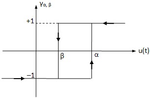Figure 1. Preisach elementary operator.

(2)

where U⁺ and U^- represent the positive and negative saturation values of input respectively. The positive Parameter a is the rise constant of the kernel and is chosen based on the discrete implementation explained later.

If C[0,T] denotes the space of continuous piecewise monotone functions on the interval [0,T], then the elementary KP hysteresis operator is a mapping as following:

where ξ_p , parameterized by p, represents the initial condition of the kernel and memory the previous extreme output of kernel, and y[0,T] is the function space of output. Indeed, for a specified u(t) the KP operator Kp(u, ξ_p) maps points p(p₁,p₂) to the interval [-1,1] and is given by:

(3)

where r(x) is Lipschitz continuous ridge function. It should be mentioned that whenever the rate of input u(t) change sign, the value of memory variable ξ_p(t), depending on the kernel k_p, is updated. As mentioned formerly, time continuity of an operator is very important for physical considerations, while the parametric continuity is just useful for designing well-posed identification methodologies[19]. It was proved in[20] that for a fixed input, the KP kernel has continuity in time domain as well as in parameter space. These advantages enable the KP model as a more effective practical model to formulate and model the smart material hysteresis behavior.

The nondecreasing continuous ridge function can get any form but it is popular to select it as a continuous piecewise linear function defined as following:

(4)

Based on the above equations the KP elementary operator is depicted in figure. 2. By comparing the Preisach elementary operator and KP operator it is clear that unlike the Preisach kernel with only two branches, the KP kernel consists of a family of curves that are bounded by the curves r(u-p₂) and r(u-p₁) as shown in figure. 2. The envelope curves r(u-p₂) and r(u-p₁) link at p₁ and p₂+a . As the input u(t) varies with time, the kernel output will either track along a horizontal line between the two envelope curves r(u-p₂) and r(u-p₁), or along one of the these bounding curves.

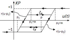Figure 2. KP elementary operator.

The Krasnosel’skii-Pokrovskii (KP) hysteresis model can be expressed as an integral of KP kernels over the Preisach plane by:

(5)

where μ(p₁,p₂) is the density of kernel KP which is utilized to weight the output of kernel KP. It means that each point p(p₁,p₂) in the Preisach plane P is associated with a specific kernel and has a specific density value μ(p₁,p₂). Therefore, the KP hysteresis model can be interpreted as a parallel connection of an infinite number of weighted kernels (figure. 3). It is reasonable to consider μ(p₁,p₂)≥0 which will automatically ensure monotone output on monotone input, provided r(x) is nondecreasing[19]. It should be mentioned here that since every KP kernels can be expressed an integration of infinite weighted Preisach relays, the KP kernel provides more information of the nonlinearity than the Preisach operator. Also, the KP model, due to its kernel, has the memory effect to record all previous extremes of the hysteresis input-output behavior. Therefore, the KP model has this facility to use less elements than Preisach model to accurately model the hysteresis behavior of smart materials.

It should be mentioned here that since the KP hysteresis model is a subclass of the classical Preisach model, the wiping-out property and the congruency property constitute the necessary and sufficient conditions for a hysteresis nonlinearity to be represented by this model. Hughes and Wen[10] demonstrated that the conditions of an SMA can be satisfied with these properties. It was concluded that the wiping-out property holds to a significant extent for the SMA actuators, while the congruency property was not completely satisfied. However, the deviation was not significant. This may, to some extent, affect the behavior prediction accuracy of the hysteresis of the SMA actuators using the classical Preisach model or KP model.

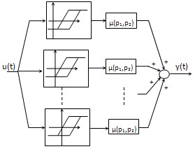Figure 3. KP model as parallel connection of weighted kernels.

It should be mentioned here that since the KP hysteresis model is a subclass of the classical Preisach model, the wiping-out property and the congruency property constitute the necessary and sufficient conditions for a hysteresis nonlinearity to be represented by this model. Hughes and Wen[10] demonstrated that the conditions of an SMA can be satisfied with these properties. It was concluded that the wiping-out property holds to a significant extent for the SMA actuators, while the congruency property was not completely satisfied. However, the deviation was not significant. This may, to some extent, affect the behavior prediction accuracy of the hysteresis of the SMA actuators using the classical Preisach model or KP model.

3. Linearly Parameterized KP Hysteresis Model

Although the first form of the KP model was first presented as equation (5) but for numerical implementing it on a real system or process there are some difficulties to calculate the hysteresis output. First of all, due to the nonlinearity nature of the kernel it is impossible to describe the outputs of the kernel as a continuous function. Second, it is a difficult task to formulate a proper weighting function which is double-integrable over the Preisach plane[22].

In order to numerically implementing the KP model, equation (5) must be transformed into parameterized form by dividing the Preisach plane P, as shown in figure. 4, into a mesh grid. If the Preisach plane P is uniformly divided by l horizontal lines and l vertical lines, then the number of small cells representing the Preisach plane P is N=0.5(l+2)(l+1). If l is selected large enough, the discretization becomes very fine and the cells become very small resulting to the parameterized KP model acts like the integral KP model. However, the computational cost become expensive forcing us to consider a suitable l. The coordinates of lower-left nodes of each cells expressed as:

(6)

where

(7)

and

(8)

is the interval of the divided input u(t). The numerical identification experiments in[27] suggested that, for the representation of hysteresis using the parameterized KP model, the optimal value of the rise constant, a, of equation (4) should be selected as , so that the kernels overlap cell by cell to create the smoothest hysteresis curves.

After discretization of the Preisach plane P we can consider the total contribution of each cell to the KP hysteresis model (5) to be lumped together as the effect of the kernel associated with the lower-left node of the cell. Therefore, one has:

(9)

where is the kernel associated with the lower left node of the cell and is called the lumped density of the ijth cell to its lower-left node with coordinate. By combining equation (5) and (9) one has:

(10)

Therefore, after parameterization the integral form of the KP hysteresis model, equation (5), it is reduced to the following form:

(11)

where

(12)

and

(13)

Vectors K and Y are called kernel vector and density vector, respectively. The term d(u(t)) is the modeling error resulted from the parameterization process. As it is mentioned before if the number of grid lines (l) increases to large value this term approaches to zero. In order to model a specified hysteresis system by the linearly parameterized KP hysteresis model, according to equation (11), its parameters (density vector Y) must identified in advance. From the practical view first the output experimental data of the system due to a known input must be gathered. The number of l dividing lines, which determines the precision of approximation, should be chosen upon the requirement of modeling precision before performing the test. Then by using equation (6)-(8) and observing the positive and negative saturation states form experimental data, the value of as well as are calculated and as stated before the value of the rise constant, a, of equation (4) should be selected as Δu. Since the kernels are characterized by and the rise constant, a, then they can easily be obtained afterward. Finally, by matching the experimental data to the simulated results, using an optimization method like least square method, the density vector Y can be obtained. After identification process and by using this calculated density vector, the simulated output corresponding to any input signal can easily be computed by using equation (11).

Table 1. Parameters of Flexible Aluminium Beam. Parameter Length Thickness Width Young Module Yield Stress SMA Wire Offset Distance Value 400 mm 1.27 mm 25 mm 70 GPa 410 MPa 10 mm

Table 2. Thermomechanical Parameters of SMA Wire Actuator Parameter Martensite Finish Temperature Martensite Start Temperature Austenite Start Temperature Austenite Finish Temperature Maximum Recoverable Strain Value 43.9 °C 48.4 °C 68 °C 73.75 °C 4.10 %

Figure 5. Schematic of the cantilever flexible beam set-up actuated by a SMA wire.

4. Experimental Test Set-up

Figures 5 and 6 present a PC-based experimental test set-up and its associated instruments which is used to investigate the capability of the linearly parameterized KP hysteresis model in prediction of a flexible beam behavior under a SMA wire actuation. of the beam does not change during cooling and heating process.

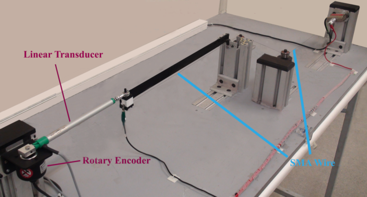Figure 6. Experimental test set-up used for verification of the current analysis results.

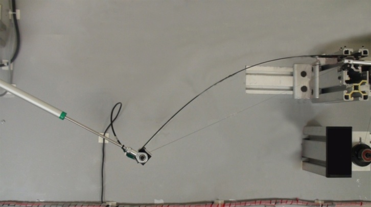Figure 7. Top view of the deformed beam after the wire actuation.

Since the tip of the beam does not move on a straight line after the SMA wire actuation, the tip of the beam is connected to a precise frictionless rectilinear displacement transducer (PZ12-A-125, GEFRAN Inc.,) while the other side of the transducer is joined to a high resolution rotary encoder (E50S series, Autonics Corporation). By measuring the length of the transducer and its angle, with respect to their initial quantities, the tip deflection of the beam can easily be computed. In addition, the output voltage of these sensors are fed to a computer-based data acquisition (not shown in figure. 6) using a AD/DA PCI multifunction card (PCI 1711, Advantech Inc.,) and Matlab Real Time Data Acquisition Toolbox (Matlab R2008a, Mathworks Ltd.,). The activation electric voltage over the SMA wire is set by the computer generated voltage controlling a voltage amplifier which is capable of delivering up to 3A current. Figure. 7 shows the top view of the deformed structure after the heating process

5. Identification and Validation Processes

The input voltage applied to the SMA actuator in the training process is a slow decaying ramp signal and is shown in figure. 8. The rate of change of the input voltage is selected so small in order to allow the temperature to stabilize, as in the steady state temperature will be determined by applied electrical voltage. In the training process of the linearly parameterized KP hysteresis model, 439 data set, consist of the major loop and 10 first order descending reversal curves attached to the major loop, is used. For identification density vector of linearly parameterized KP hysteresis model following values are used:

It should be mentioned here that if the wiping-out and congruency properties are valid, then it does not matter which transition curves are used for modeling of hysteresis nonlinearity by the Preisach or KP model and all of them will theoretically lead to the same result[2]. However, from the practical viewpoints, the first-order transition curves have some clear merits. First, it is easier to get these curves experimentally rather than higher-order transition curves. Second, measurements of these curves start from a well-defined state – the state of negative (or positive) saturation[2]. We performed the wiping out and congruency tests in this research (not reported here) and it is concluded that, same as the result of[18], the wiping-out property holds to a significant extent for our SMA actuator, while the congruency property is not completely satisfied. However, the deviation is not significant. It is worth mentioning that since the output of the system (tip deflection of the beam) never gets negative values, the ridge function (equation (4)) is corrected as following:

The switching values of the descending reversal curves are selected as: [2.4, 2, 1.8, 1.75, 1.7, 1.65, 1.6, 1.55, 1.5, 1.45, and 1.4] (volt). For switching values less than 1.4 (volt), the change in the beam deflection is not considerable. The experimental input-output hysteresis loops of the flexible beam with SMA wire actuator, under the abovementioned input voltage is shown in figure. 9.

Figure 8. The decaying ramp input voltage applied in the training process.

Figure 9. Experimental data of hysteresis behavior between the beam tip deflection and the SMA wire voltage in the training process.

For evaluation and comparing the prediction of the beam end deflection by the linearly parameterized KP hysteresis model with respect to the experimentally measured data, in the first validation process the voltage profile shown in figure. 10 is applied to the SMA actuator. It should be mentioned that although the form of the voltage applied in this validation process looks like what was applied in the training process, the extremums are different. The switching values of these descending reversal curves attached to the major loop are selected as: [2.325, 1.975, 1.725, 1.675, 1.625, 1.575, 1.525, 1.475, and 1.425] (volt). The experimental input-output hysteresis loops of the flexible beam with SMA wire actuator, under the abovementioned input voltage is also shown in figure. 11. The experimentally measured data of the beam tip deflection is compared with the prediction of the linearly parameterized KP hysteresis model in figure. 12. let's define the percentage of error as following:

Figure 10. The decaying ramp input voltage applied in the first validation process.

Figure 11. Experimental data of hysteresis behavior between the beam tip deflection and the SMA wire voltage in the first validation process.

Figure 12. Comparison between the displacement response of the linearly parameterized KP hysteresis model and the measured data of the flexible smart beam in the first validation process.

then the effectiveness of the linearly parameterized KP hysteresis can also be seen from the percentage of absolute error (%) plot, in the time domain, presented in figure. 13. As it is clear from these figures, the linearly parameterized KP hysteresis model has excellent ability in predicting the beam behavior under the voltage actuations which are same as ones implemented in the training process. In order to show this property more clearly, the maximum, mean and mean squared values of the absolute error are also presented in

Figure 13. Time history of percentage of error in the first validation process.

Table 3. Error of The Linearly Parameterized KP Hysteresis Model in First Validation Process Mean of Absolute Error (mm) Max of Absolute Error (mm) Mean of Squared Error (mm) 0.9513 17.1450 3.2029

Table. 3. Since the maximum deflection of the beam under the SMA wire actuation is 134.5 mm, the peak prediction error in this case is about 12.7% of the maximum output.

Figure 14. The input voltage profile applied in the second validation process.

For better evaluation of the linearly parameterized KP hysteresis model in predicting the beam hysteresis behavior, in the second validation process the voltage profile shown in figure. 14 is selected for actuation of SMA wire. Unlike the first validation process, this form of actuation voltage leads to some first order reversal ascending curves attached to the descending part of major loop. The experimental input-output hysteresis loops of the flexible beam with SMA wire actuator, under the abovementioned input voltage is shown in figure. 15. The switching values of these ascending reversal curves are selected as: [0.3, 0.9, 1.1, 1.15, 1.2, 1.25, 1.3, 1.35, 1.4, 1.45 and 1.5] (volt). The experimental measured displacement, as a result of this actuation voltage, is compared with the prediction of the linearly parameterized KP hysteresis model in figure. 16. The percentage of error, in the time domain, is also presented in figure. 17. The maximum, mean and mean squared values of the absolute error are also presented in Table. 4. The result clearly shows that in this validation process, in which the form of the actuation voltage differs from what is applied in the training process, the prediction of the linearly parameterized KP hysteresis model is weaker than the first validation process but acceptable.

Table 4. Error of The Linearly Parameterized KP Hysteresis Model in Second Validation Process Mean of Absolute Error (mm) Max of Absolute Error (mm) Mean of Squared Error (mm) 3.5077 23.1998 24.4681

Figure 15. Experimental data of hysteresis behavior between the beam tip deflection and the SMA wire voltage in the second validation process.

Figure 16. Comparison between the displacement response of the linearly parameterized KP hysteresis model and the measured data of the flexible smart beam in the second validation process.

Figure 17. Time history of absolute error between linearly parameterized KP hysteresis model and experimental measured displacement responses in the second validation process.

As stated before if wiping out and congruency tests are completely satisfied it does not matter which first order reversal curves (descending or ascending) are selected for the training process and all of them leads to the same results. however, since the congruency tests are not completely satisfied for the SMA materials[18] as well as our actuator and also due to the training process by first order descending reversal curves, then the linearly parameterized KP simulation results for the first order ascending reversal curves have some differences with respect to the experimental data and in this case the error are more than the first validation process. In this case the peak prediction error is about 18.2% of the maximum beam deflection.

Figure 18. The input voltage profile applied in the third validation process.

Figure 19. Comparison between the displacement response of the linearly parameterized KP hysteresis model and the measured data of the flexible smart beam in the third validation process.

Most of the phenomenological hysteresis models have difficulty in predicting higher order hysteresis minor loops and this leads to poor results when their inverse is implemented as a feedforward controller. For appraising the ability of the linearly parameterized KP hysteresis model in these situations, in the third validation process a damped voltage profile shown in figure. 18 is applied to the SMA actuator. The prediction of the higher order hysteresis minor loops by the linearly parameterized KP hysteresis model is compared with the experimentally measured data in figure. 19. The percentage of error, in time domain, is also presented in figure. 20. The maximum, mean and mean square values of the absolute error are also presented in Table. 5. The peak prediction error in this case is about 10.8% of the maximum output.

Table 5. Error of The Linearly Parameterized KP Hysteresis Model in Third Validation Process Mean of Absolute Error (mm) Max of Absolute Error (mm) Mean of Squared Error (mm) 2.5593 14.5554 11.7153

Figure 20. Time history of absolute error between the linearly parameterized KP hysteresis model and experimental measured displacement responses in the third validation process.

As it was expected and it is obvious from figure. 20 and Table. 5, the linearly parameterized KP hysteresis model has moderate accuracy in predicting the higher order hysteresis minor loops especially when, like this case, it has been only trained with some first order hysteresis reversal curves attached to the major loop. The close match between the simulation result and the experimental data shows that the linearly parameterized KP model works well for predicting higher order hysteresis curves of the SMA actuator system.

6. Conclusions

The Preisach model is one of the powerful operator-based phenomenological models which is used in modeling complex hysteretic nonlinear behavior in shape memory alloy actuators. In order to have continuous operator in time domain as well as in parameter space Krasnosel’ skii- Pokrovskii [12] allows the Preisach kernels to be any reasonable functions. The KP type operator, a special case of a so-called generalized play operator, is a hysteretic operator treating continuous branches rather than jump discontinuities like in the Preisach operator.

Since the original integral form of the KP model easily cannot numerically and practically implemented, the linearly parameterized KP model usually applied. In this method, a finite number of the kernel functions is utilized and each kernel function itself stands for a reasonable approximation of actual hysteresis curves of the actuator.

In most of the researches conducted about the modeling of SMA actuators by KP model, only the ability of the KP model in characterizing the hysteretic behavior of the actuators is demonstrated with respect to some specified experimental data and the accuracy of the developed model with respect to other data is not validated. In other words only the parameters of KP model are identified in order to adapt the model response to the real hysteretic nonlinearity with some specific experimental data and finally the outputs of the obtained KP are compared with those same data. Therefore, it is not clear whether the developed model is capable of predicting hysteresis minor loops of SMA materials or not and how its accuracy in this prediction task is. This issue is important from this point of view that if the inverse of the KP model is a candidate for hysteresis nonlinearity compensation using an open loop feedforward controller, it is important to know how accurate the developed model would model the observed input-output relation and determine whether using a feedback controller is essential or not.

In this paper, first the parameterized KP model is identified by some experimental data obtained from an experimental test set-up consisting of a flexible beam actuated by a shape memory alloy wire. The training data are 439 data set, consist of the major loop and 10 first order descending reversal curves attached to the major loop. The parameters of the KP model are identified by least square method in order to adapt the model response to the real hysteretic nonlinearity. Then the accuracy of the developed KP model with known parameters in predicting nonlinear hysteretic behavior of first order ascending curves and higher order minor loops, is validated with some other experimental data. Although the model has been trained with data of first order descending reversal curves, it has good power in behavior prediction of first order ascending curves as well as higher order minor loops. The maximum prediction error of the developed model in characterizing the first order ascending curves and higher order minor loops are, respectively, 18.2% and 10.8% of the maximum output. In order to achieve better results more data should be applied. According to result of this paper and it is a good candidate for predicting the hysteresis nonlinearity of SMA actuators as well as a feedforward controller to compensate the hysteretic nonlinearity behavior of SMA actuated structures.

ACKNOWLEDGEMENTS

The authors would like to thank Eng. Ali Vahedi, manager of Nanotechnology and Smart Structure Group in HESA aeronautical research center for his great supports. Thanks are also extended to HESA Simulators & Flight Training Systems for helping with the construction of the experimental test set-up used in this paper. Authors also appreciate research scholar Hamid Salehi for many valuable comments.