1. Introduction

In the framework of the standard Galerkin/Ritz method for the solution of one-dimensional boundary value problems governed by a differential equation within the domain [0,L], the usual procedure consists of subdividing [0,L] into a certain number of finite elements for which piecewise-linear (i.e., local) interpolation is assumed[1]. In general, the shortest the elements are the more accurate the numerical solution is (h-version). Alternatively, higher order p-methods[2] suggest the introduction of nodeless basis functions based on differences of Legendre polynomials (up to the seventh degree) that cooperate with the two linear shape functions, i.e., , the latter associated to the ends x = 0 and x = L. A literature survey suggests that for a certain discretization of the domain, the corresponding p-version is generally more accurate than the h-version[3-6].

The matter of using higher order approximations through computer-aided-design (CAD) based Coons-Gordon macroelements has been recently discussed for two- and three-dimensional problems[7-11]. In those works some similarities and differences of the so-called ‘Coons macroelements’ with respect to the ‘higher order p-method’ have been reported in detail. Moreover, alternative CAD based NURBS or/and Bézier techniques have been proposed within the last eighteen years[12-16].

In this context, this paper continues the investigation on the eigenvalue problem by moving from 2-D and 3-D to 1-D eigenvalue problems, and seeks for any similarities or essential differences between five alternative methods. The study includes classical Lagrange polynomials and extends to the Bernstein polynomials that are inherent in the definition of Bézier CAD curves[17], as well as to Chebyshev polynomials that have been previously used in spectral and collocation methods (e.g.[18]). In this paper it was found that all the aforementioned polynomials are equivalent in the sense that (after the proper transformation) they symbolically coincide with the classical higher order p-method (or p-version)[2] as well as with the class (Taylor series).

2. Galerkin/Ritz Formulation

2.1. General

A general Sturm-Liouville problem can be written in the following differential equation

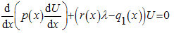It can be reduced to a study of the canonical Liouville normal form

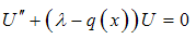(1)

Without loss of generality, in this paper we deal with the particular case that, for which Eq(1) degenerates to the well-known ‘Helmholtz equation’:

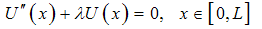(2)

Equation (2) covers many practical problems in physics and engineering such as the axial elastic vibrations of a beam or the sound propagation along a straight acoustic pipe.

The solution of Eq(2) is usually expressed as a series expansion in two alternative ways:

(3a)

(3b)

where f_i (x) are the basis functions and a_j the generalized co-ordinates that refer to n+1 nodeless parameters. Also, N_j(x) are the shape functions and U_j the nodal displacements at the positions x=x_j , j=0,…,n. It is reminded that N_j(x) are cardinal functions, i.e. N_j(X_i)=δ_ij (= Kronecker’s delta) and also partition the unity, i.e.

for all. There are also some formulations in which both shape and basis functions participate such as higher order p-methods[2].

In any case, the Galerkin/Ritz procedure[1] consists first of the Galerkin method, i.e.

with denoting the weighting function, and second by the partial integration of the second order term, which finally leads to the alternative matrix formulations:

(4a)

(4b)

where the elements of the mass () and stiffness () matrices are given by:

(5a)

(5b)

2.2. Basis Functions and Shape Functions

Below, occasionally either the Cartesian coordinate or its normalized value will be used. It is well known that any interval [a, b] can be reduced to[0,1] by a simple change of variable.

2.2.1. First Degree (Linear) Finite Element

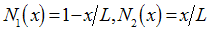
According to the standard literature[1], for a finite element of length l_k, the two linear shape functions, that is, are associated to the ends x = 0 and x = l_k. It is well known[1] that the basis functions related to the aforementioned shape functions are: and, that is.

2.2.2. Lagrangian Type Macroelement

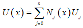
The domain [0,L] is subdivided into n (preferably equidistant) segments, thus leading to nodes. Then, the variable U is globally interpolated within the entire domain [0,L] in terms of Lagrange polynomials associated to the aforementioned nodes. For a non-decreasing sequence of points, , the Lagrange polynomial is defined as:

(6)

giving unity at and passing through n points. Typical sets of Lagrange polynomials are shown in Table 1. Therefore, Equation (3a) holds with denoting the jth Lagrange polynomial (). As for each k the denominator in Eq(6) is a constant, whereas the nominator is a polynomial of degree n, the latter can be written in terms of its roots

() as follows:

Table 1. Lagrange polynomials of low degree (1 ≤ n ≤ 4).

2.2.3. Bernstein Polynomials

According to standard computer-aided-geometry knowledge, for example[17], a Bézier curve of n-th degree is defined in terms of the normalized coordinate as

(7)

In standard mathematical texts the variable in Eq(7) is called “Bernstein polynomial of degree n” and is denoted by [19, p. 36], whereas the basis or blending functions, , are named “Bernstein basis” and are defined as

(8)

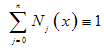
The geometrical coefficients, , are called control points. Equation (8) denotes that for a curve that is defined by (n + 1) control points, the highest degree is, which means that the degree of a Bézier curve is defined by the number of control points. It has been shown that Bernstein polynomials have the property of partition of unity and also the first () and the last of them () give unity at the first () and the last end () of the interval [0,1], respectively. It is remarkable that at any internal control point is less than the unity [17], and also vanishes at the endpoints u = 0, 1. It is trivial to prove that, at least for the case of a straight segment, when the interval [0,L] is uniformly divided into a number of so-called breakpoints, the control points coincide with them.

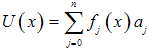
Following the ideas of CAD/CAE integration previously proposed by the author in the context of closely related isoparametric Coons interpolation[7-11] as well as the “isogeometric” idea of Hughes et al.[14] referring to NURBS representation, in this work we propose to substitute the Cartesian coordinate in Eq.(7) by the variable. Therefore, with respect to Eq.(3b), the basis functions correspond to and also the control points are replaced by the coefficients.

2.2.4. Higher Order P-Method

Following Szabó and Babuška[2], the variable is expanded to a series like that in Eq(3b). According to this technique [2, p.38], the two first basis functions, which correspond to x=0 and x=L, are identical with the linear shape functions associated to the end points of the entire interval [0,L], i.e., and and are called nodal shape functions. The rest (n-1) basis functions are called internal shape functions and are taken as suitable integrals of Legendre polynomials properly multiplied by specific coefficients dependent on the ascending order. It must become clear that the latter refer to nodeless quantities (general coefficients) and, therefore, they are also called “bubble modes”.

By elaborating on [2], in cases of n = 2, 3 and 4, the bubble basis functions are given by ():

(9b)

(9c)

2.2.5. Chebyshev Polynomials

Chebyshev polynomials are categorized as first and second kind.

I. First kind

(10a)

II. Second kind

(10b)

2.2.6. General Remarks

From the above analysis, it becomes obvious that Lagrange, Bernstein, Legendre, and Chebyshev polynomials are different options with the following characteristics:

I. Lagrange polynomials are cardinal shape functions that operate directly on the nodal values,.

II. Bernstein (basis) polynomials are generally non-cardinal basis functions. The only exception are the two basis functions, and, which are associated to the ends (x = 0, x = L); thus they operate directly on the nodal boundary values and. The remaining coefficients are associated to the internal control points.

III. Legendre polynomials create bubble basis functions that operate on nodeless generalized coefficients, a.

IV. Chebyshev polynomials (both of first and second kind) differ from the above cases in the sense that they neither become unit nor vanish at the ends of the domain.

A careful inspection of all above five polynomial interpolations [Eqs.(6),(8),(9) and (10)], and considering the well known binomial expansion, it is easily concluded that all these polynomials can be expanded in a Taylor (power) series of the form:

(11)

For each of the five abovementioned polynomials, different coefficients [Eq(11)] are derived.

2.2.7. Special Cases

In order to bring insight in the topic of subsection 2.2.6, some special cases of small size will be discussed in full detail.

I. First, in the first four (Lagrange, Bernstein, P-method, Chebyshev of 1^st kind) alternative types of polynomials, the case of using only one segment for the discretization (n = 1) is strictly related to the linear interpolation between the two endpoints. Therefore, the same classical finite element matrices, which are given below by Eq.(12a) and (12b), are obtained. For Chebyshev of 2nd kind (), the factor “2” in induces a slight modification.

II. Second, in the case of two subdivisions, equivalent polynomials which include terms up to the second degree, is represented in Table 2. From Table 2, it becomes obvious that all functional sets are complete, as they include all the terms of the set {1, u, u2}. Moreover, while Lagrange and Bernstein (basis) polynomials ensure the partition of unity (rigid body) property, the p-method and Chebyshev polynomials do not.

3. Analytically Calculated Matrices

Based on Eqs(5), the stiffness and mass matrices are analytically calculated through manipulation and are shown below.

3.1. Linear Interpolation (n = 1)

In this case, all three formulations of this paper degenerate to the simple case of the conventional linear finite element of the literature[1]. The matrices are given by:

(12)

where denotes the length of the finite element. It is well known that accuracy increases when the total length L of the domain is divided into an increasing number of such elements (h-version). In this case, the total mass and stiffness matrices are obtained from the assemblage of all finite elements involved [1].

3.2. Quadratic Approximation (n = 2)

The relevant matrices are:

1. Lagrange polynomials:

(13a)

2. Bernstein polynomials:

(13b)

3. Higher order P-method:

(13c)

3.3. Cubic Approximation (n = 3)

Based on Eqs(5), the stiffness and mass matrices are given by:

1. Lagrange polynomials:

(14a)

2. Bernstein polynomials:

(14b)

3. Higher order P-method:

(14c)

One can notice that in the case of the p-method, no symmetry exists along the diagonal terms of the mass matrix which correspond to internal modes (). This fact can be explained on the basis of Table 3, where one can notice that the shape functions and of Lagrange and Bernstein polynomials are symmetric with respect to the central point u=1/2, while the same does not hold for the p-method.

3.4. Quartic Approximation (n = 4)

Based on Eqs(5), the stiffness and mass matrices are given by:

1. Lagrange polynomials:

(15a)

2. Bernstein polynomials:

(15b)

3. Higher order P-method:

(15c)

One can notice that in the case of the p-method, again no symmetry exists along the diagonal terms of the mass matrix which correspond to internal modes ().

Table 2. Alternative polynomials involved in case of n = 2 (series expansion is included in the lower row).

Table 3. Alternative polynomials involved in case of n = 3.

3.5. Chebyshev Polynomial Based Matrices

Below we present the matrices for the most general case dealt in this study, which is for the quartic approximation (). Obviously, for any other m < 4, the upper left submatrix should be taken ().

3.5.1. Chebyshev Polynomial of First Kind

(15d)

3.5.2. Chebyshev Polynomial of Second Kind

(15e)

3.6. Implementation of the Boundary Conditions

In this two-point boundary value problem, three alternative types of boundary conditions may exist, as follows:

i). Free-free (F-F) boundary conditions:

(16a)

ii). Both ends under Dirichlet (D-D) boundary conditions:

(16b)

iii). One end under Dirichlet, the other free (D-F):

(16c)

In general, the mathematical problem becomes:

(17)

It is well known that for small problems Eq(17) can be solved even through the characteristic polynomial, whereas for large-scale problems it is usually elaborated using any known algorithm such as subspace iteration, Lanczos, QR, etc.

Details about the treatment of boundary conditions will be discussed in Section 4.

4. Numerical Results

The domain [0, L] is subjected to either of boundary conditions (b.c.) given by Equations (16) at x = 0 and at x = L. For simplicity, the computations were performed for.

According to the boundary conditions, the exact eigenvalues are:

(i) Free-free b.c. (F-F):

(18a)

(ii) Both ends under Dirichlet b.c. (D-D):

(18b)

(iii) One end fixed (Dirichlet b.c.), the other free (D-F):

(18c)

All numerical and symbolic (Symbolic Toolbox) calculations were performed on a PC (DELL Latitude E6500) using MATLAB 7.12.0 (R2011a). Given the stiffness K and mass matrices M, the symbolic eigenvalues were found using the command eig(inv(M)*K), whereas the alternative command eig(K,M) works for the numerical operations only.

For a given polynomial of degree n, the error norm of the i-th calculated eigenvalue is determined as:

(19)

4.1. Free-Free (F-F) Boundary Conditions

This case requires no special care as none row or column has to be eliminated.

In all six cases, i.e. (i) Lagrange, (ii) Bernstein, (iii) p-method, (iv) Chebyshev of 1st kind, (v) Chebyshev of 2nd kind, and finally (vi) Taylor series, the eigenvalues were found to be identical. Moreover, the convergence quality is excellent (the same quality with the results presented in Table 4) but it is not presented for the sake of briefness.

4.2. One Dirichlet (D-F) or Two Dirichlet (D-D) Boundary Conditions

For the last two types of boundary conditions [D-D and D-F: Eq(16)b,c], and for the first three types of polynomials [i.e. (i) Lagrange, (ii) Bernstein, and (iii) p-method], the row(s) and column(s) that correspond to the restricted end(s) is (are) simply eliminated. As previously happened, in all these three types of polynomials the eigenvalues were found to be identical. Moreover, convergence quality is shown in Table 4, labeled as D-D and D-F.

In contrast, in case of either Chebyshev polynomials or Taylor series the way of elimination of row(s) and column(s) is not apparent yet.

5. A Theoretical Explanation

Since all types of polynomials dealt in this study [i.e. (i) Lagrange, (ii) Bernstein, (iii) p-method and relevant Legendre polynomials, as well as (iv) Chebyshev of first and (v) Chebyshev of second kind] span the basis functions included in the class (Taylor power series):

(20)

Table 4. Calculated eigenvalues using polynomials of nth degree (n uniform subdivisions). Results are shown as errors (in %) for two support conditions: (a) both ends are fixed (D-D), and (b) one end is fixed and the other is free (D-F).

5.1. The Class

In this case the variable U is expanded in a Taylor series:

(21)

According to Eq.(5b), the elements of the mass and stiffness matrices will be given by:

(22)

5.2. A Proof for the Identical Eigenvalues

For a single square matrix of order (n+1), Ralston and Rabinowitz[19, p. 484] (Theorem 10.3) have demonstrated that any similarity transformation applied to leaves the eigenvalues of the matrix unchanged. The same is found in the textbook of Bathe [20, p. 45] where, provided is orthogonal, a poof is given through the characteristic polynomial.

In this paper we generalize the proof to any pair of stiffness and mass matrices (Theorem 3); the upper left superscript ‘’ takes the symbolic values ‘t’, ‘l’, ‘b’, ‘p’ as well as ‘c1’ and ‘c2’, which correspond to the initials of the six alternative polynomials (Taylor series, Lagrange polynomials, Bernstein basis, P-method/Legendre, as well as Chebyshev of 1^st and 2^nd kind). Theorem 1 and Theorem 2 aim to support Theorem 3.

THEOREM-1. The change of basis between a basis polynomial [such as Lagrange, Bernstein, P-method, Chebyshev et cetera], and the class (Taylor series), induces a relationship of quadratic form between the mass matrices and.

PROOF.

First, we consider the basis vectors of order (n+1), for both abovementioned functional sets:

(23)

Based on Eq(23), the corresponding mass matrices [cf. Eq(5b)] are given in compact form as follows:

(24)

Second, we consider the equivalent expressions of U(x) using either Taylor series or the μ-type polynomial basis, for which it holds:

(25)

Since U(x) is a scalar, it equals to its transpose, therefore:

(26)

Left-multiplication of Eq(25) by Eq(24) in parts, leads to:

(27)

Integrating the last two parts of Eq(27) over the interval [0,L], and considering that the vectors and are constant (so they can exit the integral), we obtain:

(28)

Substituting Eq(24) into Eq(28), one obtains the desired matrix identity:

(29)

Equation (29) constitutes the proof of the theorem.

Remark: It is reminded that Eq(29) is the well known matrix transformation (from local to global system) in the finite element praxis (e.g., [1,20]). Nevertheless, in this study only mathematical considerations have been taken into account, whereas in engineering books it is usually derived on the basis of virtual work (the latter is considered to be invariable in both local and global orthogonal co-ordinate systems). In contrast, in this work no orthogonality relationship between the different bases was considered.

THEOREM-2. The contents of Theorem-1 is extended to the stiffness matrices and as well.

PROOF.

Taking the derivatives in x of the vectors in Eq(23), we obtain the two new vectors:

(23a)

Therefore, the corresponding stiffness matrix [Eq(5b)] is written as:

(24a)

Henceforth the proof is the same as in Theorem-1, leading to the identity:

(30)

THEOREM-3. For any pair of matrices (,), which corresponds to a basis polynomial, the corresponding eigenvalues are identical with the eigenvalues, of the pair (,) that is produced by the class (Taylor series).

PROOF.

Considering the stiffness and mass matrices [Eq(22)], the reference eigenvalue problem becomes (stands for the coefficients in Taylor series):

(31)

Furthermore, considering the stiffness and mass matrices, the new eigenvalue problem becomes (stands for the corresponding coefficients in -type polynomial basis):

(32)

By left-multiplying Eq(31) by we obtain:

(33)

Equations (29) and (30) of Theorems 1 and 2, respectively, are generally applicable and therefore they hold even for the i-th eigenvector. Under these circumstances, substituting them into Eq(33) we obtain:

(34)

By left-multiplying Eq(24) by, one obtains:

(35)

Finally, subtracting Eq(34) and eq(35) in parts, one obtains:

(36)

Since the quadratic form cannot vanish, it is concluded that:

(37)

which constitutes the proof of the theorem.

Corollary. The identical eigenvalues can be expressed by common Rayleigh quotients:

(38)

5.3. Application of Arbitrary Boundary Conditions

Whatever follows is generally applicable but for the purposes of this paper it has particular value for Taylor series and Chebyshev polynomials, which do not directly apply for the boundary conditions.

Equation (25) is collocated at (n + 1) points within the interval [0,L]. One possible, but not restrictive possibility is to uniformly divide the domain [0,L] into n segments, thus introducing the breakpoints:

(39)

Therefore, we derive a relationship in the form:

(40)

which in vector form is written as:

(40a)

or equivalently:

(41)

Substituting Eq(41) into Eq(35) we derive:

(42)

where

(43)

In this framework, it is now trivial in Eq(42) to eliminate the row and column that corresponds to the Dirichlet boundary condition.

6. Discussion

The motivation of this work was the interesting paper by Çelik[18] that deals with the collocation method using Chebyshev polynomials, which constitute a complete functional set. Previously, the state-of-the-art was the use of basis functions in the form of algebraic polynomials in the form, with and, so as to ensure satisfaction of the homogeneous Dirichlet boundary conditions in the interval [a,b] (for example, [21]).

At that period the author had accumulated numerical experience on the excellent behavior of global approximation, either using B-splines or Lagrange polynomials ([7-11], among others). Later, when he tried to compare the eigenvalues obtained using (i) Lagrange polynomials, (ii) Bernstein (basis) ones, and (iii) Taylor series, a numerical coincidence was remarked when the same collocation points were used [22].

The abovementioned numerical coincidence pushed the author to extend his research from collocation to the most popular finite element method in which closed form analytical formulas of the matrices can be derived. In this formulation, not only the previously found coincidence[22] was repeated, but also it was further found that the famous P-method[2] is also identical with all others.

Although one could simply state that all these polynomials (Lagrange, Bernstein, Legendre, and Chebyshev) have the same basic basis, which is the class (Taylor series), the possible statement that the Rayleigh quotient is the same has to be mathematically proven.

Another interesting point is the way that the boundary conditions are imposed. As previously mentioned, Lagrange polynomials are associated directly to the nodal values of the primary variable U all-over the domain, whereas the Bernstein (basis) polynomials refer to control points. However, since the extreme control points, P₀ and P_n, coincide with the two ends, there is no problem to impose free-free or Dirichlet boundary conditions. Similarly, the p-method is based on the well known linear shape functions associated to the ends of the interval [a,b], and simply its functional set is enriched by the nodeless bubble functions.

In contrast to the two aforementioned polynomials, similar to the Taylor series, Chebyshev polynomials have a more spectral character, as they refer to arbitrary coefficients instead of the pure values of the variable U, i.e. U₀ and U_n. It is worthy to mention a common characteristic similarity between Chebyshev polynomials and P-method. In more details, as the degree n of the polynomial increases, the stiffness matrix K_n and mass matix M_n (both of order (n+1)) can be immediately derived from the previously calculated submatrices K_n-1 and M_n-1 (both of order n), by simply completing the (n+1)-th row and the (n+1)-th column (it is reminded that in Section 2 the indices vary between 0,…,n).

Despite the coincidence found in one-dimensional problems, preliminary comparisons in two-and three-dimensional problems suggest that there is a significant difference between Lagrangian type finite elements and the p-method, as the first occupy a broader space than the second ones [9,10].

7. Conclusions

In this work, the entire one-dimensional domain [0,L] was considered as a single macroelement (global approximation), at the ends of which three (all possible) different types of boundary conditions were imposed. Also, for the spatial approximation of the variable U five different types of global higher order polynomials were considered. It was found that all these five basis functions, i.e. (i) classical Lagrange polynomials, (ii) Bernstein polynomials (useful in CAD curve representation), (iii) bubble functions based on Legendre polynomials (p-method), as well as Chebyshev polynomials of (iv) first kind and (v) second kind, share the same functional space, i.e.. Although the coefficients of series expansions and relevant matrices highly depend on the particular polynomial chosen, the calculated eigenvalues were found always the same, a fact that was also rigorously proven initially in case of free-free and then for arbitrary boundary conditions.