1. Introduction

Stochastic systems frequently possess structural specifications that are hard to represent mathematically [1-5]. While “optimal” conditions can be calculated for the mathematical formulations, whether these solutions are actually the best for the original “real” system design conditions is far less certain [1], [2], [6]. To improve the decision-making process when faced with such ambiguities, it often proves preferable to propose a few dissimilar options that represent different system perspectives [3], [7]. To be beneficial to the system designers, these distinct options need to be close-to-optimal with respect to their mathematically modelled objective(s), but maximally different from each other within the solution space [6-8]. The primary purpose behind this alternative generation approach is to construct a set of dissimilar options that are “good” when evaluated with respect to the specified system objective(s), but which are fundamentally different from each other in the decision domain. The system designers then need to perform a subsequent assessment of this set of alternatives to determine which specific option(s) most closely satisfy their situation. Consequently, this approach is considered as a decision support method rather than as the solution creation process assumed in “normal” mathematical optimization.

Earlier option formulation approaches employed a straightforward process in which each alternative was incrementally constructed by re-running the solution creation algorithm whenever a new option needed to be produced [6-10]. These iterative procedures mimicked the seminal approach in [8] where, after the initial mathematical model had been optimized, all supplementary alternatives were produced one-at-a-time. These incremental approaches all employed n+1 computational iterations – initially to optimize the original problem, then to produce each of the subsequent n alternatives [7], [11-18]. Subsequently, it was demonstrated how a set of maximally different alternatives could be efficiently generated using any population-based algorithm by permitting the generation of the overall optimal solution together with n distinct alternatives in a single computational run irrespective of the value of n [19-23]. In [24] a data structure was created that permits alternatives to be constructed simultaneously by population-based solution methods.

In this paper, it is demonstrated how a set of maximally different system design options can be produced by extending several earlier techniques into stochastic optimization ([12-18]). This stochastic approach advances the earlier procedures ([13,15-18]) by permitting the simultaneous generation of n distinct alternatives in a single computational run. Namely, to construct the requisite n maximally different system design options, the algorithm has to run only once irrespective of the value of n [19-23]. Furthermore, a bicriteria, max-sum, max-min objective is employed that combines the novel data structure into the simultaneous solution algorithm. The efficacy of this approach is illustrated on a water resources management system case study.

2. Generating Distinct Solution Options

Mathematical programming has focused almost exclusively on finding single optimal solutions to single-objective problems or, equivalently, producing noninferior solutions to multi-objective formulations [2], [5], [8]. While these approaches may solve the formulations as constructed mathematically, whether these solutions are truly “best” for the original “real world” applications remains less certain [1], [2], [6], [8]. In most “real world” systems, there are countless system specifications that can never be incorporated into the mathematical problem formulation [1], [5]. Unavoidably, the majority of the subjective aspects remain unmodelled and unquantified in the mathematical system formulations. This frequently occurs when final outcomes are decided upon based not only on modelled objectives, but also on more subjective socio-political-economic preferences and stakeholder goals [7]. When unmodelled components are suspected to exist, non-traditional solution approaches are needed for searching the decision space not only for noninferior solutions, but also for sub-optimal possibilities. Specifically, any search for alternatives to problems suspected to possess unmodelled components must concentrate not only on a non-inferior set of solutions, but also necessarily on an explicit exploration of the problem’s inferior solution space. Numerous “real life” instances of these types of modelling situations are illustrated in [6], [8], [9], and [10].

To demonstrate the impact of unmodelled objectives on a solution search, assume that the optimal solution to a maximization problem is X* with objective value Z1* [24]. Suppose a second, unmodelled, maximization objective Z2 exists that represents some “politically acceptable” feature. Assume that the solution, X^a, belonging to the 2-objective noninferior set, exists that corresponds to a best compromise solution if both objectives could actually have been simultaneously considered. While X^a would be the best solution to the real problem, in the actual mathematical formulation it would seem inferior to solution X*, since Z1^a Z1*. Thus, when unmodelled components are included in the decision-making process, inferior decisions to the mathematically modelled system could actually be optimal to the fundamental “real” problem. If unmodelled aspects and unquantified objectives might exist, alternative solution procedures are essential to not only explore the decision region for noninferior solutions to the modelled problem, but also to concurrently search the decision space for explicitly inferior solutions.

Necessarily, then, in these situations, the aim is to create a workable set of options that are quantifiably good with respect to the modelled objectives yet are as different as possible from each other within the solution space. By satisfying this maximal difference condition, the resulting set of alternatives is able to supply truly different perspectives that all perform similarly with respect to the known modelled objective(s) yet very differently with respect to various potentially unmodelled aspects. By creating good-but-different options, the system designers are the able to consider potentially desirable qualities within the alternatives that might be able to satisfy the unmodelled objectives to varying degrees of stakeholder acceptability.

To motivate the process, it is necessary to formally characterize the mathematical definition of maximal difference [6], [7]. Assume that the optimal solution to an original mathematical programming formulation is X* with corresponding objective value Z* = F(X*). An ensuing difference model can then be solved to produce an alternative solution, X, that is maximally different from X*:

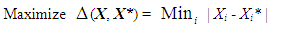(1)

(2)

(3)

where represents an appropriate difference function (shown in (1) as an absolute difference) and T is a tolerance target relative to the original optimal objective value Z*. T is a user-specified limit that determines what proportion of the inferior region needs to be explored for acceptable alternatives. This difference function concept can be extended into a difference measure between any set of alternatives by replacing X* in the objective of the maximal difference model and calculating the overall minimum absolute difference (or some other function) of the pairwise comparisons between corresponding variables in each pair of alternatives – subject to the condition that each alternative is feasible and falls within the specified tolerance constraint.

The population-based procedure that is subsequently employed is designed to generate a fixed, pre-determined number of close-to-optimal, but maximally different alternatives, by adjusting the value of T and solving the corresponding maximal difference problem instance by exploiting the population structures of the optimization algorithm. The survival of solutions depends upon how well the solutions perform with respect to the problem’s originally modelled objective(s) and simultaneously by how far away they are from all of the other alternatives generated in the decision space.

3. Stochastic Optimization via Simulation

Finding optimal solutions to large stochastic problems proves complicated when numerous system uncertainties must be directly incorporated into the solution procedures ([25-28]). In the stochastic optimization via simulation procedures considered in this study, all uncertain parameters, constraints, and objective functions are replaced by simulation models in which the decision variables provide the settings under which simulation is performed. The basic stages can be summarized in the ensuing way ([26], [29]). Assume that the mathematical formulation of the optimization problem consists of n decision variables, , denoted by the vector 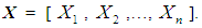If the objective is given by the function F and the feasible region is designated by D, then the mathematical programming problem is to optimize F(X) subject to X D. When stochastic conditions exist, values for the objective and constraints are determined via simulation. A comparison between two different solutions X1 and X2 requires the evaluation of some statistic of F modelled with X1 compared to the same statistic modelled with X2 ([25], [30]). These statistics are calculated via simulation, in which each X provides the decision variable settings employed in the simulation. While simulation provides the context for comparing results, it does not provide the mechanism for finding optimal solutions to problems. Hence, simulation alone cannot be used for stochastic optimization purposes.

Since the measures of system performance are stochastic, each potential solution, X, is evaluated from simulation. Because simulation is computationally intensive, an optimization procedure is used to direct the search for solutions through the problem’s feasible region in as few simulation runs as possible ([27], [30]). As stochastic system problems frequently contain potentially numerous feasible solutions, the quality of the final solution could be exceedingly variable unless an extensive search has been performed throughout all portions of the feasible space. Necessarily, the stochastic optimization method contains two alternating computational phases; (i) an “evolutionary” phase directed by some optimization method (frequently a metaheuristic) and (ii) the solution simulation phase ([31]). Because of the stochastic components, all performance measures are necessarily statistics calculated from the responses generated in the simulation phase. The quality of each solution is found by having its performance criterion, F, evaluated in the simulation phase. After simulating each candidate solution, their respective objective values are returned to the evolutionary phase to be utilized in the creation of the succeeding candidate solutions. Thus, the evolutionary phase aims to advance the system toward improved solutions in subsequent generations and ensures that the solution search does not become trapped in some local optima. After generating new candidate solutions in the evolutionary phase, the new solution set is returned to the simulation phase for comparative evaluation. This alternating, two-phase search process terminates when an appropriately stable system state (i.e. an optimal solution) has been attained. The optimal solution produced by the procedure is the single best solution found throughout the course of the entire search process ([31]).

Population-based optimization methods are particularly beneficial for these types of searches because the complete set of candidate solutions maintained within their populations permit searches to be undertaken throughout multiple sections of the feasible region, concurrently. For population-based optimization methods, the evolutionary phase evaluates the entire current population of solutions during each generation of the search and evolves from a current population to a subsequent one. An evolutionary characteristic of population-based procedures is that better solutions in a current population possess a greater likelihood for survival and progression into the subsequent population.

It has been shown that this type of optimization-via-simulation approach can be used as a very computationally intensive, stochastic technique ([30], [32]). However, because of the very long computational runs, several approaches to accelerate the search times and solution quality have been explored [29]. The next section introduces a procedure that incorporates simulated stochastic uncertainty to much more efficiently generate sets of maximally different solution options.

4. Stochastic Bicriteria Algorithm

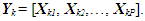
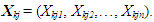
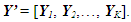
In this section, a previously introduced data structure is used that permits the stochastic bicriteria algorithm to be employed for creating system options using any population-based solution algorithm [24], [33-36]. Suppose that the goal is to produce P distinct options in which each individual option possesses n decision variables and the algorithm’s population is to possess K sets of solution alternatives overall. Therefore, each solution in the population contains one complete set of P maximally different alternatives. Let Y_k, k = 1,…, K, represent the k^th solution consisting of one complete set of P different alternatives. Specifically, if X_kp is the p^th alternative, p = 1,…, P, of solution k, k = 1,…, K, then Y_k can be represented as

(4)

If X_kjq, q = 1,…, n, is the q^th variable in the j^th alternative of solution k, then

(5)

Accordingly, the entire population, Y, comprised of K different sets of P alternatives can be expressed in vectorized format as,

(6)

The following stochastic method can produce a pre-determined number of close-to-optimal, maximally different system options, by modifying the value of T in the maximal difference model and using any population-based optimization algorithm to solve the corresponding, maximal difference problem. Each solution in the population is composed of one complete set of P different possible system options. By exploiting the co-evolutionary aspects of the algorithm, the procedure evolves each solution (i.e. set of alternatives) toward sets of dissimilar local optima within the solution domain. In this processing, each solution alternative mutually experiences the search steps of the algorithm. Solution survival depends both upon how well the solutions perform with respect to the modelled objective(s) and by how far apart they are from every other alternative in the decision space.

A straightforward process for generating alternatives would iteratively solve the maximum difference model by incrementing the target T whenever a new alternative needed to be produced and then re-solving the updated model [24]. This iterative approach parallels the seminal Hop, Skip, and Jump (HSJ) approach [8] in which the alternatives are constructed one-at-a-time through an incremental adjustment of the target constraint. Although the HSJ is straightforward, it necessitates a repetitive execution of the optimization algorithm [7], [12], [13]. To improve upon the stepwise HSJ approach, a concurrent technique was subsequently designed based upon co-evolution ([13], [15], [17]). In a co-evolutionary approach, pre-specified stratified subpopulation ranges within an algorithm’s overall population are established that collectively evolve the search toward the specified number of maximally different alternatives. Each desired solution alternative is represented by each respective subpopulation and each subpopulation undergoes the common processing operations of the procedure. The survival of solutions in each subpopulation depends simultaneously upon how well the solutions perform with respect to the modelled objective(s) and by how far away they are from all the other alternatives. Consequently, the evolution of solutions in each subpopulation toward local optima is directly influenced by those solutions contained in all of the other subpopulations, which forces the concurrent co-evolution of each subpopulation towards good but maximally distant regions within the decision space according to the maximal difference model [7]. Co-evolution is more computationally efficient than the sequential HSJ-style approach by exploiting inherent population-based searches to concurrently generate the entire set of maximally different solutions using only a single population [12], [17].

While concurrent approaches possess the ability to exploit population-based algorithms, co-evolution can only occur within each of the stratified subpopulations. Consequently, the maximal differences between solutions in different subpopulations can only be based upon aggregate subpopulation measures. Conversely, in the following stochastic algorithm, each solution in the population contains exactly one entire set of alternatives and the maximal difference is calculated only for that particular solution (i.e. the specific alternative set contained within that solution in the population). Hence, by the evolutionary nature of the population-based search procedure, in the subsequent approach, the maximal difference is calculated simultaneously for the specific set of alternatives considered within each specific solution – and the need for concurrent subpopulation aggregation measures is circumvented.

Using the data structure terminology, the steps for the stochastic bicriteria algorithm are as follows ([14], [19-24], [33-36]). It should be readily apparent that the stratification approach employed by this method can be easily modified for solution via any population-based optimization algorithm.

Initialization Step. Solve the original optimization problem to find its optimal solution, X*. Based upon the objective value F(X*), establish P target values. P represents the desired number of maximally different alternatives to be generated within prescribed target deviations from the X*. Note: The value for P must be fixed a priori by the decision-maker.

Without loss of generality, it is possible to skip this step and to use the algorithm to find X* as part of its solution processing in the subsequent steps. However, this significantly increases the number of iterations of the computational procedure and the initial stages of the processing become devoted to finding X* while the other elements of each population solution are retained as essentially “computational overhead”.

Step 1. Create an initial population of size K where each solution contains P equally-sized partitions. The partition size corresponds to the number of decision variables in the original optimization problem. X_kp represents the p^th alternative, p = 1,…,P, in solution Y_k, k = 1,…,K.

Step 2. In each of the K solutions, evaluate each X_kp, p = 1,…,P, with respect to the modelled objective using simulation. Alternatives meeting both their target constraint and all the other problem constraints are designated as feasible, while all other alternatives are designated as infeasible.

Note: An individual solution can be designated as feasible only if all of the alternatives contained within it are feasible.

Step 3. Apply an appropriate elitism operator to each solution to rank order the best individuals in the population. The best solution is the feasible solution containing the most distant set of alternatives in the decision space (the distance measures are defined in Step 5).

Note: Because the best-solution-to-date is always retained in the population throughout each iteration, at least one solution will always remain feasible. A feasible solution for the first step can always consists of P repetitions of X*.

Step 4. Stop the algorithm if the prescribed termination criteria (such as maximum number of iterations or some measure of solution convergence) are met. Otherwise, proceed to Step 5.

Step 5. For each solution Y_k, k = 1,…, K, calculate D¹_k and D²_k, which are the bicriteria Max-Min and Max-Sum distance measures determined, respectively, between all the alternatives contained within the solution.

As an illustrative example for calculating the bicriteria distance measures, compute

(7)

and

(8)

D¹_k denotes the minimum absolute distance and D²_k represents the overall absolute deviation between all the alternatives contained within solution k.

Alternatively, distance functions could be calculated using other appropriately defined measures.

Step 6. Rank order the specific solutions by those solutions which contain the set of options which are most distant from each other. The goal of maximal difference is to force the options to be as far apart as possible in the decision space from the alternatives of each of the partitions within each solution.

Let D_k = G(D¹_k, D²_k) represent the bicriteria objective for solution k. Rank the solutions according to the distance measure D_k objective – appropriately adjusted to incorporate any constraint violation penalties for infeasible solutions.

Step 7. Apply the algorithmic change operations to each solution within the population and return to Step 2.

5. Water Resources Case Study

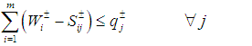
When faced with situations containing numerous uncertainties, water resources management (WRM) decision-makers often prefer to select from a set of “near best” alternatives that differ significantly from each other in terms of the system structures characterized by their decision variables. The efficacy of the stochastic bicriteria MGA algorithm will be illustrated using a WRM systems case taken from [37]. While this section briefly summarizes the case, more explicit details, data, and descriptions can be found in [37].

Maqsood et al. ([37]) previously examined a WRM problem for allocating water in a dry season from an unregulated reservoir to three categories of users: (i) a municipality, (ii) an industrial concern, and (iii) an agricultural sector. The industrial concern and agricultural sector were undergoing significant expansion and needed to know the quantities of water they could reasonably expect. If insufficient water was available, these entities would be forced to curtail their capital expansion plans. If the promised water was delivered, it would contribute positive net benefits to the local economy per unit of water allocated. However, if the water was not delivered, the results would reduce the net benefits to the users.

The major problems under these circumstances involved (i) how to effectively allocate water to the three user groups in order to achieve maximum net benefits under the uncertain conditions and (ii) how to incorporate the water policies in terms of allowable amounts within this planning problem with the least risk of system disruption. Included within these decisions is a determination of which one of the multiple possible pathways that the water would flow through in reaching the users. It is further possible to subdivide the various water streams with each resulting substream sent to a different user. Since cost differences from operating the facilities at different capacity levels produce economies of scale, decisions have to be made to determine how much water should be sent along each flow pathway to each user type. Therefore, any single policy option can be composed of a combination of many decisions regarding which facilities received water and what quantities of water would be sent to each user type. All of these decisions were compounded by overriding system uncertainties regarding the seasonal water flows and their likelihoods.

The WRM case considers how to effectively allocate the water to the three user groups in order to derive maximum net benefits under the elements of uncertainty and how to incorporate water policies in terms of allowable amounts within this planning problem with the least risk for causing system disruption. Since the uncertainties could be expressed collectively as interval estimates, probability distributions and uncertainty membership functions, the approach of [37] provided a solution for the WRM problem with a net benefit of $2.02 million.

In the region studied, the municipal, industrial, and agricultural water demands have been increasing due to population and economic growth. Because of this, it is necessary to ensure that the different water users know where they stand by providing information that is needed to make decisions for various activities and investments. For example, farmers who know there is only a small chance of receiving sufficient water in a dry season are not likely to make major investment in irrigation infrastructure. Similarly, industries are not likely to promote developments of projects that are water intensive knowing that they will have to limit their water consumption. If the promised water cannot be delivered due to insufficiency, the users will have to either obtain water from more expensive alternate sources or curtail their development plans. For example, municipal residents may have to curtail watering of lawns, industries may have to reduce production levels or increase water recycling rates, and farmers may not be able to conduct irrigation as planned. These impacts will result in increased costs or decreased benefits in relation to the regional development. It is thus desired that the available water be effectively allocated to minimize any associated penalties. Thus, the problem can be formulated as maximizing the expected value of the net system benefits. Based upon the local water management policies, a quantity of water can be pre-defined for each user. If this quantity is delivered, it will result in net benefits; however, if not delivered, the system will then be subject to penalties.

The WRM authority is responsible for allocating water to each of the municipality, the industrial concerns, and the agricultural sector. As the quantity of stream flows from the reservoir are uncertain, the problem is formulated as a stochastic programming problem. This stochastic programming model can account for the uncertainties in water availability. However, uncertainties may also exist in other parameters such as benefits, costs and water-allocation targets. In the formulation, penalties are imposed when policies that have been expressed as targets are violated. Also, within the model, any uncertain parameter A is represented by and its corresponding values are generated via probability distributions. To reflect all of these uncertainties, the following stochastic programming model was constructed by [37]:

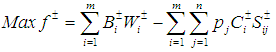(9)

(10)

(11)

(12)

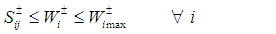
In this formulation represents the net system benefit ($/m³) and represents the net benefit to user i per m³ of water allocated ($). is the fixed allocation amount (m³) for water that is promised to user i, while is the maximum allowable amount (m³) that can be allocated to user i. The loss to user i per m³ of water not delivered is given by , where corresponds to the shortage of water, which is the amount (m³) by which W_i is not met when the seasonal flow is q_j. 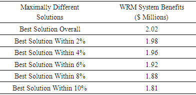is the amount (m³) of seasonal flow with p_j probability of occurrence under j flow level, where p_j provides the probability (%) of occurrence of flow level j. The variable i, i = 1, 2, 3, designates the water user, where i = 1 for municipal, 2 for industrial, and 3 for agricultural. The value of j, j = 1, 2, 3, is used to delineate the flow level, where j = 1 represents low flows, 2 represents medium flows, and 3 represents high flows. Finally, m is the total number of water users and n is the total number of flow levels.

WRM planners faced with difficult and controversial choices generally prefer to select from a set of near-optimal alternatives that differ significantly from each other in terms of their system structures. In order to create these alternative planning options for the WRM system, it would be possible to place extra target constraints into the original model which would force the generation of solutions that were different from their respective, initial optimal solutions. Suppose for example that five additional planning alternative options were created through the inclusion of a technical constraint on the objective function that decreased the total system benefits of the original model from 2% up to 10% in increments of 2%. By adding these incremental target constraints to the original SO model and sequentially resolving the problem 5 times, it would be possible to create a specific number of alternative policies for WRM planning.

However, to improve upon the process of running five separate additional instances of the computationally intensive SO algorithm to generate these solutions, the population-based, dual-criterion MGA procedure described in the previous section was run only once, thereby producing the 5 additional alternatives shown in Table 1. The table shows the overall system benefits for the 5 maximally different options generated. Given the performance bounds established for the objective in each problem instance, the decision-makers can feel reassured by the stated performance for each of these options while also being aware that the perspectives provided by the set of dissimilar decision variable structures are as different from each other as is feasibly possible. Hence, if there are stakeholders with incompatible standpoints holding diametrically opposing viewpoints, the policy-makers can perform an assessment of these different options without being myopically constrained by a single overriding perspective based solely upon the objective value.

Table 1. System Benefits ($ Millions) for 6 Maximally Different Alternatives

The computational example highlights several important aspects with respect to the MGA technique: (i) Population-based algorithms can be effectively employed as the underlying optimization search procedure for SO routines; (ii) Population-based solution searches can simultaneously generate more good alternatives than planners would be able to create using other MGA approaches; (iii) By the design of the MGA algorithm, the alternatives generated are good for planning purposes since all of their structures are guaranteed to be as mutually and maximally different from each other as possible (i.e. these differences are not just simply different from the overall optimal solution as in an HSJ-style approach to MGA); (iv) The approach is very computationally efficient since it need only be run once to generate its entire set of multiple, good solution alternatives (i.e. to generate n maximally different solution alternatives, the MGA algorithm would need to be run exactly the same number of times that the FA would need to be run for function optimization purposes alone – namely once – irrespective of the value of n); and, (v) The best overall solutions produced by the MGA procedure will be identical to the best overall solutions that would be produced for function optimization purposes alone.

6. Conclusions

Stochastic system design inherently involves unquantifiable structural elements and inconsistent design specifications. These system design problems frequently possess incompatible components that are difficult to incorporate into underlying mathematical decision models. These stochastic models frequently omit certain key system aspects that can significantly impact the appropriateness of their solutions. These omitted features require system designers to somehow incorporate numerous inconsistencies into their decision-making process prior to the final design resolution. When confronted by these incongruencies, it is unlikely that any single solution can satisfy all of the ambiguous system requirements. Consequently, decision support approaches have been created to address the confounding features, while simultaneously retaining enough flexibility to incorporate the inherent system incongruities.

This paper has applied a stochastic bicriteria procedure to system design. This computationally efficient algorithm can simultaneously construct entire sets of close-to-optimal, maximally different system design options. The bicriteria objective can efficiently generate the requisite set of good-but-dissimilar options, with each generated solution providing an entirely different perspective for the system. The max-sum objective criteria ensure that the distances between the created options are good in general, while the max-min criteria ensure that the distances between the options are good in the worst case. Since the stochastic algorithm can be applied to a wide range of system design problem, the practicality of this bicriteria algorithm can be extended to wide array of “real world” system applications. These extensions will be examined in future computational studies.