Gang Liu
Technology Research Department, Macrofrontier, Elmhurst, New York
Correspondence to: Gang Liu , Technology Research Department, Macrofrontier, Elmhurst, New York.
| Email: |  |
Copyright © 2014 Scientific & Academic Publishing. All Rights Reserved.
Abstract
We present a closed-form solution for convex Nonlinear Programming (NLP). It is closed-form solution if all the constraints are linear, quadratic, or homogeneous. It is polynomial when applied to convex NLP. It gives exact optimal solution when applied to LP. The T-forward method moves forward inside the feasible region with a T-shape path toward the increasing direction of the objective function. Each T-forward move reduces the residual feasible region at least by half. The T-forward method can solve an LP with 10,000 variables within seconds, while other existing LP algorithms will take millions of years to solve the same problem if run on a computer with 1GHz processor.
Keywords:
Nonlinear programming, Linear programming, Quadratic programming, Interior point, Simplex, Polyhedron, polynomial, Closed-form solution, Basic feasible solution
Cite this paper: Gang Liu , T-Forward Method: A Closed-Form Solution and Polynomial Time Approach for Convex Nonlinear Programming, Algorithms Research , Vol. 3 No. 1, 2014, pp. 1-25. doi: 10.5923/j.algorithms.20140301.01.
1. Introduction
A standard nonlinear optimization problem (NLP) can be formulated as: 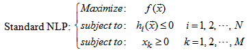 | (1) |
Which involves  variables and
  constraints. Generic NLP is hard to solve. It has been divided into several sub-set problems. Linear programming (LP) is one of the simplest sub-set of NLP, and has got concentrations for researchers. During World War II, Dantzig and Motzkin first developed the simplex method, which has become one of the most famous algorithm since then [12]. The Journal Computing in Science and Engineering listed the simplex algorithm as one of the top 10 algorithms of the twentieth century [5].Khachiyan proposed ellipsoid method in 1979[10, 11]. In 1984, Karmarkar started the so called interior-point revolution (See e.g. [9, 17]). There are also other successful algorithms for LP, such as primal-dual interior point method [13], logarithmic method [14], etc. Most of the algorithms that are successful in LP have been extended to NLP, especially the interior-point method [3], primal-dual method [6, 8], barrier methods[7, 15], all have found their roles for solving NLP. Currently, most of the LP or NLP algorithms are varieties of simplex or interior-point methods [4, 16]. Most of the current existing LP algorithms as well as NLP algorithms are path oriented and matrix oriented [1, 2]. Path oriented algorithm tries to search the optimal solution in the set of Basic Feasible Solution (BFS), which is the set of all feasible region defined by all of the constraints. However, the BFS is not obvious, thus needs to be calculated or maintained repeatedly. To maintain or to calculate BFS is one of the major difficulties and takes most of the running time for those algorithms. Also, the path oriented algorithm needs to search vertex by vertex along the edges. It could result a long path or ends up with a loop. Another common property for those existing algorithms is matrix oriented, which includes a lot of matrix operations in finding the basic feasible solutions. Convergence and exactness are two of the most important factors for an LP or NLP algorithm. Simplex method can give exact optimal solution in general. However, it is not guaranteed to give solution at polynomial time. Ellipsoid method guarantees a polynomial upper bound on convergence at the order
 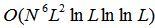 [10], and interior point method improved the convergence time to
 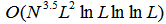 [9]. However, these polynomial time algorithms may give -approximated solution, instead of exact optimal solution. People are still looking for new methods with better convergence and can give exact optimal solution.We present a new approach, T-forward method, which can solve NLP in polynomial time with convergence speed
  , and can give exact optimal solution when applied to LP. We first construct the closed-form solution for the feasible region defined by all the constraints. Having the closed-form basic feasible solution in hand, there is no need to search paths and no need to do any matrix operations, and there is no need to save any feasible solutions in computer system. We can always get it through the closed-form formula.The closed-form solution for the BFS plays key role in the methods proposed by this paper. In fact, once we have the closed-form solution for BFS, we can transform the original optimization problem into an unconstrained problem or an equation problem. The rest of the paper is organized as follows. Section 2 discusses how to convert a generic NLP to an NLP with linear objective function. The constraints in an NLP define a feasible region. Section 3 analyzes basic concepts and properties related to a region. Section 4 analyzes the feasible region defined by a single constraint. Section 5 further analyzes the feasible region defined by all constraints and gives the closed-form solution for the feasible region for convex NLP. Section 6 gives the gradient function of the feasible region. The closed-form formulae for the feasible region and infeasible region are summarized in section 7. Section 8 introduces the concepts of the dual-point and the dual-direction. Section 9 introduces the T-Forward method, which gives closed-form solution for convex NLP. Section 10 introduces the greedy T-Forward method, which is a simplified version of the T-Forward method. Section 11 introduces the Facet-Forward method, which can solve LP in polynomial time. Section 12 gives closed-form solution for LP, Quadratic Programming, and NLP with homogeneous constraints. Section 13 presents method for solving nonconvex NLP. Section 14 gives the generic algorithm for T-Forward method. In Section 15, we apply the T-forward method to solve some example optimization problems. In Section 16, we analyze the complexity of the T-forward method and compare it with some existing LP algorithms. Conclusions are presented in Section 17.
2. Converting Generic NLP into an NLP with Linear Objective
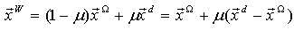
A standard NLP can always be converted into an NLP with linear objective function through the following transform: | (2) |
In fact, there should have another constraint:  . However, this constraint is redundant when we try to maximize
  . The NLP problem listed in Equation (2) is a standard NLP with Linear (NLPL) objective function. So, we only need to deal with NLP in the following format:
  | (3) |
Here, we have dropped the constraints  to make the problem more generic. If we want to include the constraints
  , we can replace
  with
with  , where
  is the set of all
  –dimensional real numbers, and is the set of all
  –dimensional real positive numbers. We may also use the following notations:
 | (4) |
 | (5) |
 | (6) |
3. Definitions Regarding a Region
The basic theory and formula in this paper are mainly based on the feasible and infeasible regions defined by the constraints within an NLPL. We first define some useful concepts or notations regarding a region  . DEFINITION: Valid path: Given a path
  , path
  is called valid path if
  . DEFINITION: Valid straight path: A valid path and the path is a straight line. DEFINITION: Connected region: A region
  is called connected region if all points in that region can be connected through a valid path.DEFINITION: Convex region: A region
  is called a convex region if any two points in region
  can be connected through a valid straight path. A convex region can be expressed in mathematics format as:
 | (7) |
Starting from any point in a convex region, we can reach any other points in that region through a valid straight path. DEFINITION: Mathematic formulation for boundary curve: A function  is called a mathematic formulation for region
  if it can be used to formulate region
  in the following format:
 | (8) |
In the rest of this section, we assume  is a mathematic formulation for region
  . DEFINITION: Boundary: If
  is formulated as the above equation, the following set
  is called the boundary of
  :
: | (9) |
DEFINITION: Shine region of a point: Given a point  , there is a region
  in which all points can be connected to
  through valid straight path.
  is called the shine region of point
  . DEFINITION: Sun shine set: Given a point set
  for
for 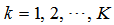 the set
  is called a sun-shine set if:
 | (10) |
That means the shine regions of a sun-shine set can cover all points in region  .DEFINITION: Order of direct connectedness: The smallest number of points of a sun-set. For example, any convex region can be shined by any point in the region, and thus the order of direct connectedness is 1. The order of direct connectedness is 1 for a circle region, and infinity for a circle line curve.DEFINITION: Ray set: Given a point
  , a unit vector
  with
with  , the ray line starting from point
  along the direction
  is called an ray set and denoted as
  .
.  can be formulated as:
 | (11) |
DEFINITION: Ray-boundary point: given a ray set  , the shortest (ordered by
  ) intersection point of
  and the boundary
  is called the ray-boundary point of the pair
  and denoted as
 . Within the ray-boundary point function,
  is called the start point,
  is called the moving direction.
  can be formulated as:
 | (12) |
Where  denotes the smallest non-zero positive root of
  in equation
 , or
, or  if it doesn’t have a positive solution. It can be expressed in mathematics format as:
 | (13) |
DEFINITION: Line region: The intersection set of  and
and  is called the line region associated to the pair of
  , and denoted as
 .
.  can be formulated as:
 | (14) |
The ray-boundary point  is the boundary point that can be reached and connected from point
  and along the direction
  .
.  is the basic function and representation for the boundary. We will try to build the
  for NLPL in following sections.
4. Regions Defined by a Constraint
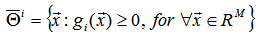
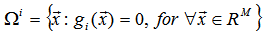
The ith constraint in the NLPL as shown in Equation (3) defines a feasible region in  . Let
. Let  denote the feasible region defined by the ith constraint in Equation (3),
  denote the infeasible region (with the boundary included even they are feasible) defined by the same constraint, and
  denote the common boundary of
  and
and  . Note that, as a convention, we allow the boundary
  to be included in both the feasible region
  and infeasible region
  . We may frequently use
  to represent the ith constraint. By definition,
  ,
,  , and
, and  can be formulated as:
 | (15) |
 | (16) |
 | (17) |
 | (18) |
 | (19) |
Given a point , if
, if  and thus
 ,
,  is called a boundary point of constraint
 , and the constraint
  is called a boundary constraint at point
 . If
. If  and thus
 ,
,  is called a feasible point to constraint
 , and the constraint
  is called a valid constraint at
 . If
. If  and thus
 ,
,  is called an infeasible point to constraint
 , and the constraint
  is called an invalid constraint at
  . A constraint
  is called a simple constraint if it has only one feasible region OR only one infeasible region. In this paper, we assume all constraints are simple constraints. The ray-boundary point
  can be formulated as:
 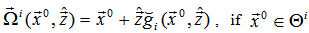 | (20) |
The above equation gives the feasible boundary point linked to point  and along the direction
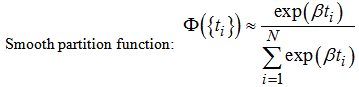
 . Figure 1. illustrates the feasible region
  and feasible boundary
  defined by a constraint in ellipsoid type.
 | Figure 1. The feasible region  and boundary and boundary  defined by a constraint in ellipsoid type. defined by a constraint in ellipsoid type.  is the gradient vector of is the gradient vector of  at point at point  |
Similarly, given a point , there should exist a region around
  in which all points are infeasible and can be connected to
  through straight line valid to
 . This region is called infeasible region connected to
  defined by constraint
 . Let
. Let  denote this region and
  denote its boundary. The ray-boundary point
  can be formulated as:
 | (21) |
5. Feasible Region Defined by All the Constraints in NLPL
All the constraints in an NLPL as shown in Equation (3) define an  –dimensional polytope in
  , which contains some piece-wise curves as its facets, and each piece-wise curve must be a part of one of the feasible boundary
  defined in NLPL. All the points in the feasible region are also called Basic Feasible Solution (BFS). Let
  denote the feasible region defined by all the constraints in NLPL,
  denote the infeasible region defined by all the constraints in the same NLPL,
  denote the common boundary of
  and
and  .
.  is the set in
  that have all the constraints satisfied. By definition, we should have:
  | (22) |
 | (23) |
 | (24) |
 | (25) |
Given a point  , there should have a region that all points can be connected to
  through a straight line valid to
  . Let
. Let  denote this region and
  denote its boundary. Similarly, given a point
  , there should have a region that all points can be connected to
  through a straight line valid to
  . Let
. Let  denote this region and
  denote its boundary. Based on our definition, both
  and
and  are convex, and
 | (26) |
 | (27) |
The line-region  can be formulated as:
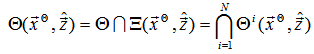 | (28) |
 | (29) |
Thus, the ray-boundary point  can be formulated as:
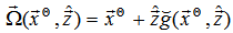 | (30) |
where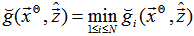 | (31) |
Note that all items within the min operation in the above equation are positive and none-zeros. Then the above equation can be equivalently transformed into: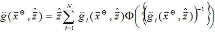 | (32) |
Where  is the following function:
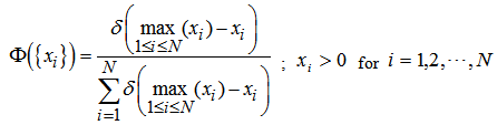 | (33) |
And  is an
is an  function defined as:
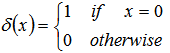 | (34) |
Function  has the following property:
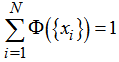 | (35) |
Then,  can be interpreted as a probability partition function of the set
  with non-zero probability when
  , and 0 probability for other cases.
  can also be expressed in the following format:
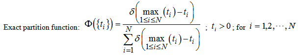
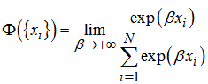 | (36) |
To make it easy for use, we can simply drop the “lim” operation by replacing  with a large number. Then, the above equation can be written as:
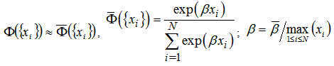 | (37) |
 is a large number such that
  is acceptable for computer system without data over flow. Normally,
  is good enough for numerical calculations.
 is called exact-partition function, whereas
  is called smooth-partition function. Here we use
  to denote the smooth format partition function, so that it can be distinguished from the exact format. In fact, they give almost the same values once
  is big enough. In the rest of the paper, as long as there is no confusion, we will use the same notation
  for both smooth and exact format partition functions. Using the partition function, the ray-boundary point
  in both exact and smooth formats becomes:
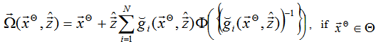 | (38) |
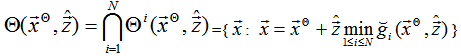
Suppose  has been solved from the equation
  for all
  , then both Equation (30) and (38) give closed-form solution for a feasible point
  , which is the ray-boundary point of
  .
.  will give all points of the shine-region
  once point
  goes through all possible directions. Further, once point
  goes through all points of a sun set,
  will give all the points on feasible boundary
  . Therefore, Equation (30), or its smooth format Equation (38), is a closed-form solution for the feasible boundary
  or BFS defined by all constraints in an NLPL.
6. Gradient Function of the Feasible Boundary
In real applications, we may frequently need the gradient of the feasible boundary  . Since we already have the closed-form solution for the feasible boundary, especially its smooth format, the gradient function can be calculated by differentiating the boundary function. However, here we give another simple method to calculate the gradient function. Keeping in mind that partition function
 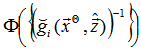 is the probability distribution function for any constraint
  to be on the boundary
  . Then, we can use the partition function as a weight or probability distribution to calculate the gradient function. Let
  denote the gradient of the feasible boundary curve
  at the point
  . Then it can be formulated as:
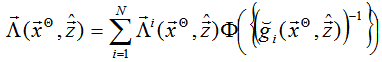 | (39) |
Where  is the unit gradient vector of the constraint curve
  at the point
  .
.  can be formulated as:
 | (40) |
 gives the average gradient of all the curves passing through the point
  on the feasible boundary
  . It could be slightly different from the gradient calculated by differentiating the boundary function. However, they will be the same as long as the corresponding boundary point contains only one constraint, which is most of the case. Although the smooth format might be slightly different from the exact format, it always gives a good approximation when
  is big enough. The exact format gradient function may not be continuous, while the smooth format is always smooth and continuous. When calculating the gradient, it would be better to use the smooth format partition function.
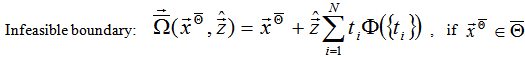
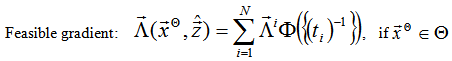
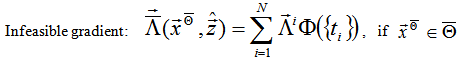
7. Summary of Equations for Boudaries Defined by All Constraints
We have formulated the closed-form solution for the feasible boundary  and its gradient. Similarly, we can construct the infeasible boundary
  and its gradient by formulating the ray point
  starting from an infeasible point
  and along the moving direction . As a summary, let us list the boundary functions and the gradient functions for
  and
and  as following:
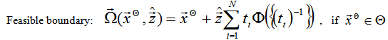 | (41) |
 | (42) |
 | (43) |
 | (44) |
Supplementary functions: | (45) |
 | (46) |
 | (47) |
 | (48) |
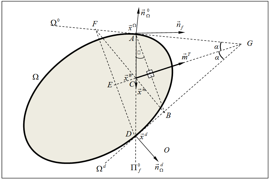
These are the major functions we are going to use in the rest of this paper. Figure 2. illustrates some vectors or points related to the boundary curve and can be calculated by the above equations. 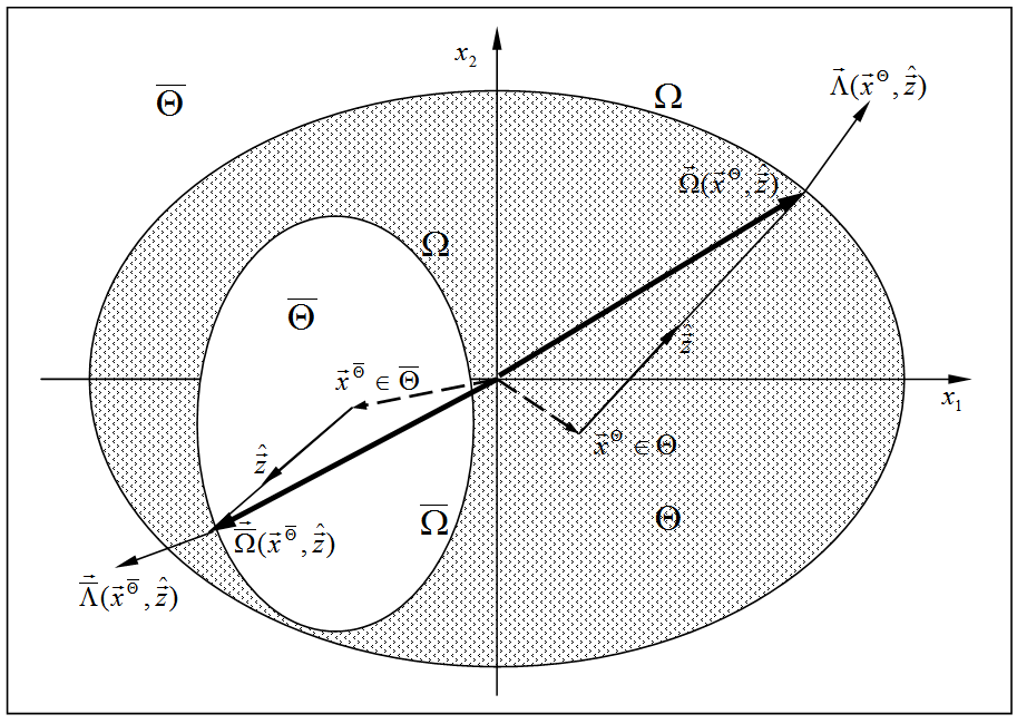 | Figure 2. The right side shows the feasible boundary  , one of its ray-boundary point , one of its ray-boundary point  , and its gradient , and its gradient  . The left side shows the infeasible boundary . The left side shows the infeasible boundary  , one of its ray-boundary point , one of its ray-boundary point  , and its gradient , and its gradient  |
8. Dual-point and Dual-direction
Using the boundary functions given in the previous section, we can start from a point  to find a feasible ray-boundary point. If
  is an infeasible point, we can apply function
  to get a feasible point. Suppose
  is a feasible boundary point we have found. Let
  denote the boundary point and the ending point of
  as shown in Figure 3. Let
  denote the contour plane of the objective function passing through point
  , which can be formulated as
  . Let
. Let  denote the unit gradient vector of
  ,
,  denote the tangent plane of the boundary
  at point
  , and
, and  denote the unit gradient vector of
  at point
  . Let vector
  be the projected vector of
  onto
onto  , point D be the intersection point of
  with
with  , C be the mid point between
  and D.Figure 3. Illustrates the points and curves mentioned above.
 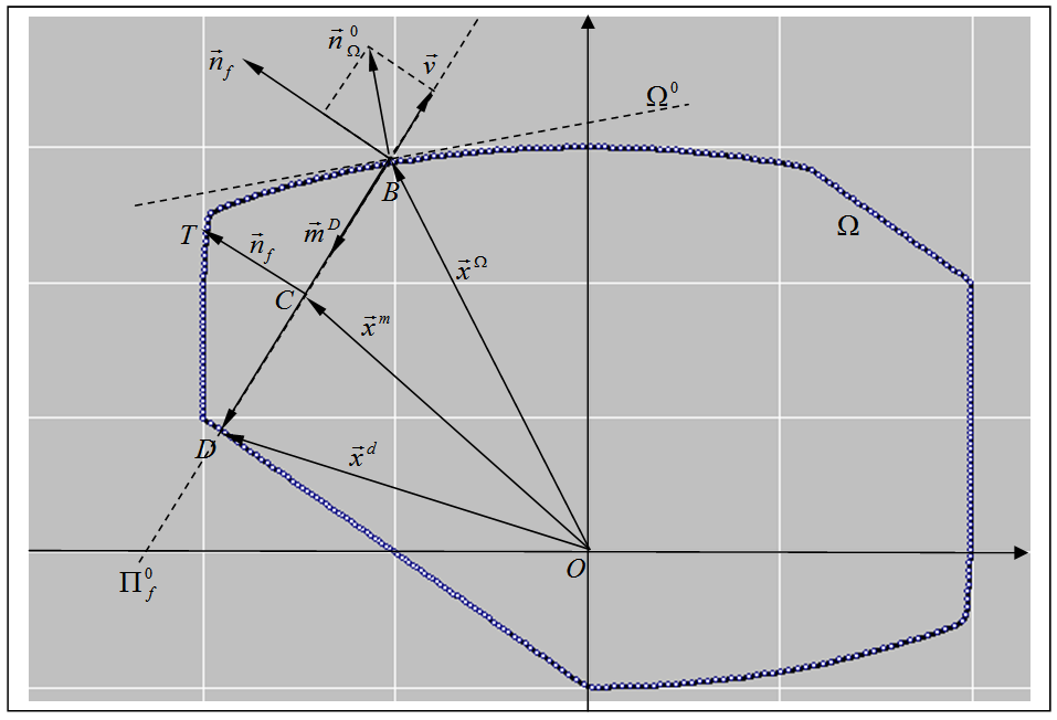 | Figure 3. A feasible boundary point  , its dual-point , its dual-point  , the mid-interior-point , the mid-interior-point  , and the dual-direction , and the dual-direction  |
DEFINITION: dual-direction. Vector 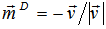 is called the dual-direction. If
  , we set the dual-direction to
  .DEFINITION: dual-point. Given a boundary point
  , its ray-boundary point along the dual-direction is called the dual point of
  , which is the point D or
  as shown in Figure 3. DEFINITION: mid-interior-point. The middle point between a boundary point
  and its dual point
  is called the mid-interior-point of
  . Here we borrow the words “interior point” and “dual point” to indicate some special points related to a boundary point and the boundary curves. However, both of them are very different form the interior-point method and the dual method that are frequently used in the optimization world.Using the boundary gradient function, the gradient vector
  can be calculated as:
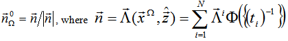 | (49) |
The dual-direction can be easily formulated as: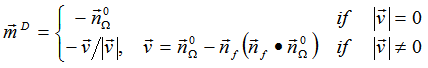 | (50) |
The dual-point can be formulated as: | (51) |
The mid-interior-point can be formulated as: | (52) |
9. T-Forward Method for Nonlinear Programming Problems
Building on the closed-form solution for the feasible boundary and for the boundary gradient, we can give a near-closed-form solution for NLP problems. Figure 4. illustrates some of the notations we are going to use in this paper and their relationships. 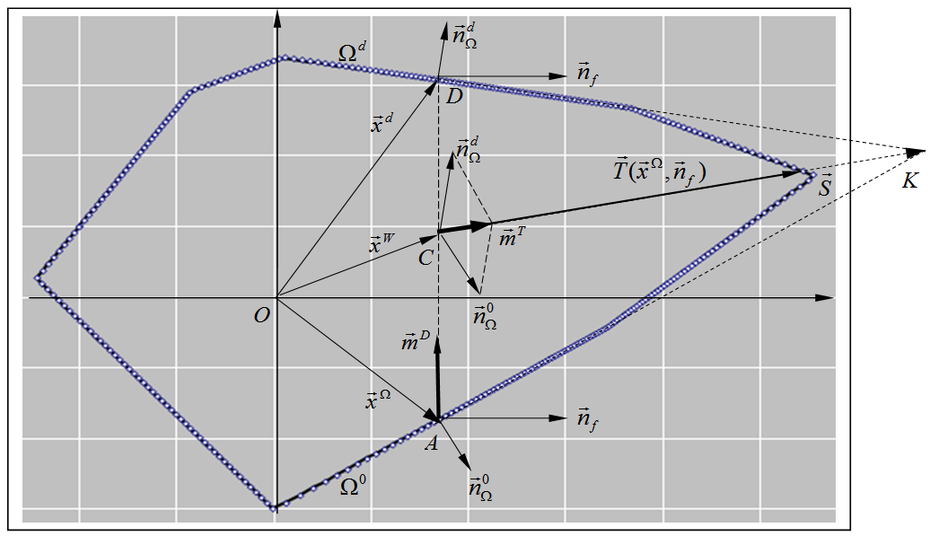 | Figure 4. Illustration of the T-Forward vector  , and how it related to the feasible boundary point , and how it related to the feasible boundary point  , the dual-point , the dual-point  , the mid-interior-point , the mid-interior-point  , the dual-direction , the dual-direction  , and the T-forward direction , and the T-forward direction  . Point . Point  is the T-forward point. Point K represents the common edge of is the T-forward point. Point K represents the common edge of  and and  |
The following notations will be used in the rest of the paper: : A feasible point,
  .
. : An infeasible point,
  .
. : A feasible boundary point,
  .
. : The gradient of the objective function.
 : The dual point of
  ,
,  .
. : The mid-interior point of
  ;
; : The tangent curve of
  at the point
  ;
; : The tangent curve of
  at the dual-point
  ;
; : The common edge of
  and
and  ;
; : The gradient of
  ;
; : The gradient of
  ;
; : The objective contour plane passing through point
  and
and  ;
; : Dual point direction,
  ;
; : T-forward direction,
  ;
; : The point that gives optimal solution to the NLPL problem; We will use
  as the basic variables and have other variables expressed as a function of the pair
  .Figure 5. Illustrates weighted-interior-point
  and how to calculate the weight
 .
. | Figure 5. Illustration of the weighted-interior-point  and the mid-interior-point and the mid-interior-point  . A is the initial point . A is the initial point  . D is the dual point . D is the dual point  . The mid-interior-point . The mid-interior-point  is at the middle of the line is at the middle of the line  . C is the weighted-interior-point . C is the weighted-interior-point  , which divides the line , which divides the line  with with  and and  as the weight factors. Starting from the point C (the end point of as the weight factors. Starting from the point C (the end point of  ), the T-forward direction ), the T-forward direction  will point to the point G, which is the common edge of the tangent curve will point to the point G, which is the common edge of the tangent curve  and the dual tangent curve and the dual tangent curve  |
DEFINITION: T-forward-direction. T-forward direction is defined as: | (53) |
DEFINITION: Weighted-interior-point  . The weighted-interior-point is defined as:
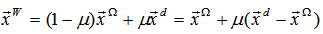 | (54) |
 | (55) |
DEFINITION: T-forward-point. The ray-boundary point starting from the weighted-interior-point  and along the T-forward direction
  is called the T-forward-point, denoted as
  .Using the weighted-interior-point as starting point and the T-forward-direction as the forward move direction, the ray-boundary-point
  will point to the point K, which is the common edge of the tangent curve
  and the dual tangent curve
 . The T-forward-point will try to reach the edge or vertex whenever possible.DEFINITION: T-forward-function: The function maps from the pair
  to the T-forward-point
  is called T-forward-function, which is also denoted as
  . By definition, the T-forward-point
  can be formulated as:
 Thus, the T-forward-point and the T-forward-function
  can be written as:
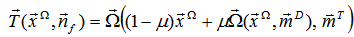 | (56) |
The T-forward point  is also a boundary point. We can apply the T-forward-function to it to get another T-forward-point. By applying the T-forward-function repeatedly, we will eventually reach a point where the T-forward-point cannot move further. That must be a point where the objective contour plane and the feasible boundary
  have just one common contact point. That is the optimal solution for the NLP in the shine-region
  . DEFINITION: T-forward-solution: Given a feasible boundary point
  and the objective gradient
  , let
, let  denote the optimal solution for the NLPL problem in the shine-region
  (with
(with  as its boundary). By repeatedly applying the T-forward-function, we can reach a solution for the NLPL. This solution is called T-forward-solution and denoted as
  . The T-forward solution can be formulated as:
 | (57) |
Or expressed in iterative format: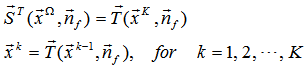 | (58) |
DEFINITION: T-forward point method: Using the T-forward-function to solve NLPL problem is called T-forward point method, or simply T-forward method. DEFINITION: T-forward path: The series of the T-forward points starting from the initial point  and ending at the optimal point
  make up a path, which is called T-forward path. DEFINITION: T-forward accuracy: The relative difference between
  and
and  is called T-forward accuracy, denoted as
  . That is:
 | (59) |
Given a feasible boundary point  , we can find its dual-point
  . Both
  and
and  are on the same contour plane
  , and thus give the same objective value. If the feasible region is convex and continuous, all the points between
  and
and  should be interior points and thus have some points between the contour plane and the feasible boundary
  . For those points that are outside the contour plane
  and along the direction
  , which is the normal direction of
  , will give better objective values. Particularly, the T-forward-point between
  , will possibly give the longest move within the feasible boundary
  if we move from
  along the direction
  . As long as the point
  is a strict interior point, the ray-boundary-point
  will definitely give a larger objective value than the point
  . Normally, T-forward-point method gives ɛ-approximated solution for NLP. For LP problems, the T-forward-point method is designed to move to the edge or vertex if possible. The final solution is always on the optimal edge or vertex. As long as the LP has a solution, the T-forward-point method guarantees to give the exact optimal solution.
10. Greedy T-Forward Method for Nonlinear Programming Problems
The Greedy T-forward method a simplified version of the T-forward method. Everything is the same as the T-forward method except it takes the mid-interior-point  as the starting point in each T-forward step. So, if we replace
  with
with  , the T-forward method will become greedy T-forward method. Compared with the T-forward method, the greedy T-forward method doesn’t have any advantages except its simplicity. It may work as efficient as the T-forward method. However, it may not give exact optimal solution when applied to LP problems. Everything in the previous section is applicable to the greedy T-forward method. There is no need to repeat them. Here we just list the greedy T-forward function. By definition, the greedy T-forward-point
  can be formulated as:
 Thus, the greedy T-forward-point and the greedy T-forward-function
  can be written as:
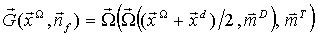 | (60) |
The greedy T-forward solution can be formulated as: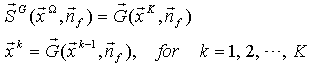 | (61) |
11. Facet-forward Method for Linear Programming
The T-forward method gives  -approximated solution for NLP, and gives exact optimal solution for LP, both in polynomial time if the feasible region is convex. However, the complexity for the T-forward method is little bit difficult to prove. In this section, we introduce facet-forward method, which simply applies the T-forward method on facet. Given a feasible boundary
  , we can find its constraint curve
  . Let
. Let  be the facet on
  and contains the point
  , that is:
 | (62) |
The facet-forward method first finds the local optimal solution of the LP problem restrained in the facet  , let it be
  . Then we cut the feasible boundary
  using the objective contour plane
  , which passes the point
  . This can be easily done by adding the function
  as an extra constraint to the original LP listed in Equation (3). Let us call the feasible boundary of the LP problem as the original feasible boundary. Once we add an objective contour plane
  to the original problem LP, the original feasible boundary
  will be cut by the contour plane
  into two parts.DEFINITION: NLPL on residual feasible region. The NLPL problem of the original problem restrained in the residual feasible boundary. In other words, it is the following NLPL problem:
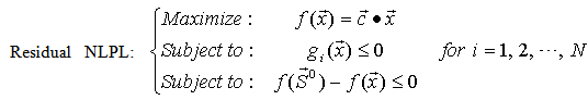 | (63) |
DEFINITION: Residual Feasible Boundary. The feasible boundary of the residual NLPL problem. Actually, it is the set of the original feasible boundary with objective value greater than  . Since
  is the largest value on the facet
  , then the constraint
  becomes completely redundant to the LP on residual feasible boundary. The constraint
  can be completely removed from the problem by substituting with the new constraint
  . The new constraint doesn’t have any impact when we search on another facet and try to find objective values greater than
  . So, the problem becomes a LP with the number of constraint reduced by at least 1. There are N constraints in total, so, at most of N steps of such facet forward search, we will find the optimal solution. One method for finding the local optimal solution within a facet is called on-boundary T-forward method. The on-boundary T-forward method simply applies the T-forward method in a facet, which means the dual point, the dual direction and the T-forward direction are all restrained in the facet. Another method is called edge-forward method. Given a staring feasible point, we can apply the ray-boundary point function
  repeatedly to the starting point
  , but with the moving direction vector
  constrained in the facet
  , sometimes may be along the edge of that facet. By repeating this process, we can eventually reach the local optimal solution of the specified facet.
12. Closed-form Solutions
Everything in the optimal solutions  as described in the previous sections are in closed-form format except the root value
  . If
. If  can also be expressed in closed-form format, then all these solutions
  give closed-form solution for NLPL or LP in the region
  . Actually, we can give closed-form solution for
  for some special cases. In this section, we give closed form solution for LP, QCQP, and NLP with Homogeneous (NLPH) constraints.
12.1. Closed-Form Solution for Linear Programming
If the problem is LP, then all constraints are linear functions. The constraint  can be expressed as:
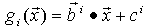 | (64) |
Then 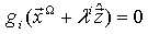 becomes:
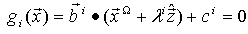 | (65) |
From which we can easily solve  as:
as: 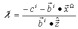 | (66) |
Based on the definition for  , we have:
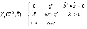 | (67) |
It is in closed-form format, and thus Equation (58) gives closed-form solution for LP. Also, the feasible boundary for LP must be convex and have just one region. Then, Equation (58) gives global optimal solution for LP.
12.2. Closed-Form Solution for Quadratically Constrained Quadratic Programming
In the case of QCQP, all the constraints are quadratic. The constraint  can be expressed as:
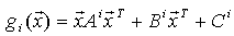 | (68) |
Then 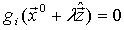 becomes:
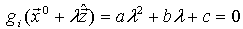 | (69) |
where | (70) |
 can be solved through the well known closed-form solution for quadratic equation:
 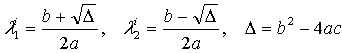 | (71) |
By definition,  can be formulated as:
 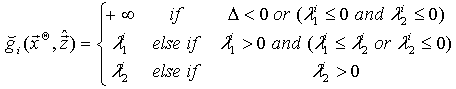 | (72) |
Then Equation (58) gives closed-form solution for QCQP.
12.3. Closed-Form Solution for NLP with Homogeneous Constraints
DEFINITION: Homogeneous function. A function  is called homogeneous with degree
  if:
if: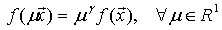 | (73) |
Here  is a positive integer number.DEFINITION: NLP with homogeneous constraint (NLPH). A nonlinear programming in which all the constraints are homogeneous. For an NLPH, the ith constraint can be expressed as:
 | (74) |
And  has the following property:
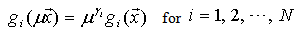 | (75) |
For an NLPH, the origin point is always a feasible point. The  is the root of the equation
  . We can choose
  . Then
  is the root of
  . With the homogeneous property,
  can be solved as:
  | (76) |
By definition,  can be formulated as:
 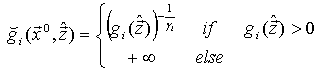 | (77) |
Therefore, Equation (58) gives the closed-form solution for NLPH.
13. Find the Global Optimal Solution for NLPL
Given a feasible point  , we can find the feasible boundary point
  by applying
  . Then, Equation (58) and (61) give the optimal solution for NLPL in the shine region
  . If
. If  happened to be the whole feasible region
  , then the solution
  given by Equation (58) is the global optimal solution for NLPL. For example, when
  is convex, we should have
  . Then
  is the global optimal solution for NLPL. Particularly, the feasible region of an LP is always convex, we can always give global optimal solution through the closed-form solution
  for LP. However, if
  cannot cover all the feasible region
  ,
,  might be a local optimal solution. In that case, we need to find a sun-shine-set that can cover all points in the feasible region through direct path connection. The infeasible boundary function
  given in Equation (42) can be useful in finding the sun-shine set. Suppose
  , we can apply
  with some randomly generated directions
  until we find a feasible point that is not in the shine regions that have been searched.
14. Algorithm for T-Forward Method
Based on the previous sections, the algorithm for T-Forward method can be summarized as follows. Main Procedure: T-forward-method Input:
  : requested precision; N: number of the constraints; M: Number of variables;
  : gradient of the objective function;
  : an feasible interior point; and all the coefficients in each of the constraint
  .Output: A feasible boundary point
  that maximizes the objective function.1. Formulate the original NLP in the following NLPL as shown in Equation :
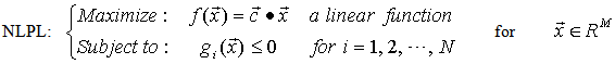 2. Initialization 2.1. Set
  2.2. Set
  2.3. Calculate ray-boundary point
 get-ray-boundary-point
 2.4. Set
 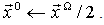 3. While
  do loop3.1. Set
  3.2. Set
  get-T-forward-point
 3.3. End While-do loop.4. Return
  as the optimal solution and
  as the optimal objective value. End of T-forward-method
 Function get-T-forward-point
 Input: A boundary point
  , and all the input information for the NLPL.Output: A boundary point
  , which is the T-forward point with
  as starting point.1. Set
  2. Calculate
  for the point
 get-partition-function
 3. Calculate gradient vector
 get-gradient-vector
 4. Calculate dual point
  through Equation :
 get-dual-point
 5. Calculate gradient vector
 get-gradient-vector
 6. Calculate T-forward direction
  through Equation :
 7. Calculate weighted-interior point
  through Equation :
 ;
;  ;
;  8. Calculate T-forward point
  :
: get-ray-boundary-point
  End of Function get-T-forward -point
 Function get-ray-boundary-point (
 ) Input: A feasible interior or boundary point
  , a unit vector
  , and all the input information for the NLPL.Output: A boundary point
  .1. Calculate
  for the pair
 get-partition-function (
 );2. Calculate ray-boundary point
  through Equation :
 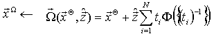 End of Function get-ray-boundary-point
 Function get-gradient-vector (
 ) Input: A boundary point
  , a unit vector
  , and all the input information for NLPL.Output:
  , which is the gradient vector of the feasible boundary at
  .1. Calculate
  for the pair
 get-partition-function
 2. Calculate gradient vector
  for each constraint at the point
  through Equation :
 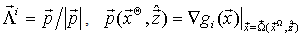 3. Calculate gradient vector
  through Equation :
 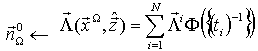 End of Function get-gradient-vector
 Function get-dual-point (
 ) Input: A boundary point
  , and all the input information for the NLPL.Output: A boundary point
  , which is the dual point of
  .1. Calculate gradient vector
  :
:  get-gradient-vector (
 ) 2. Calculate dual direction
  through Equation :
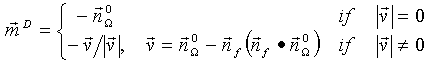 3. Calculate dual point
  :
: get-ray-boundary-point (
 )End of Function get-dual-point
 Function get-partition-function (
 ) Input: A feasible point
 , a unit vector
 , and all the input information for the NLPL.Output:
  , which is the partition function at the feasible boundary point
 .1. Calculate
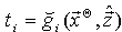 . For linear constraints,
  can be calculated through Equation (66) and (67). For quadratic constraints,
  can be calculated through Equation (70), (71), and (72).2. Calculate
  through Equation (45), (46), or (47). End of Function get-partition-function
15. Solving Linear Programming Examples
A standard LP can be expressed as: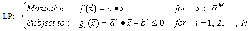 | (78) |
DFINITION: Negative Constraint. A constraint in the format  is called a negative constraint if
  , and a positive constraint if otherwise. A negative constraint is a valid constraint at the origin point. If all constraints are negative constraints, then the origin point will be a feasible point. If the origin point O is a feasible point, then, all constraints must be negative constraints. Suppose
  is a feasible point we have found, for example, we can apply simplex phase-I to find a feasible point. We can transform all constraints into negative constraints through the following transform:
 | (79) |
Then the original problem listed in Equation (78) becomes: | (80) |
 | (81) |
Without losing generality, we can assume that the LP problem has been transformed into an LP with all negative constraints. In other words, we assume the LP listed in Equation (78) has the following property: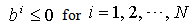 | (82) |
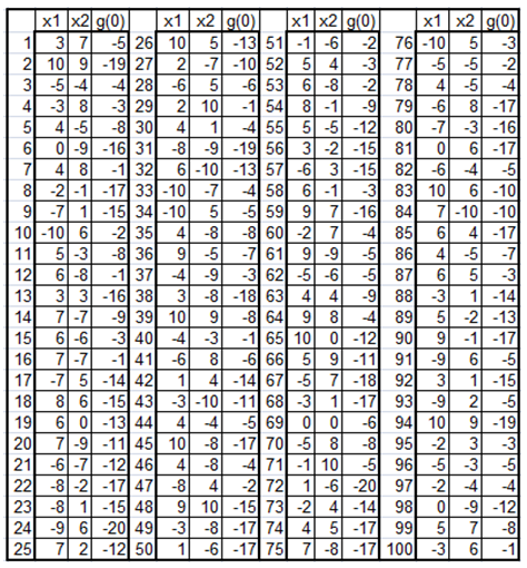
15.1. Example 1: An LP with 2 Variables and 100 Constraints
Our first example is an LP with 2 variables and 100 constraints. The input data are randomly generated numbers in the range [-10, 10] for  , and in the range [-20,-10] for
  . Table 1 lists the input data in table format.
 Table 1. Input data for LP Example-1 in table format
 |
| |
|
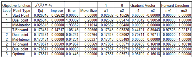
We first apply the closed-form solution, as listed Equation (41), to draw the feasible boundary  , as shown in Figure 6. It can be observed that the feasible boundary contains only 7 straight lines. Then we know that there are about 93 constraints are redundant for this problem! However, there is no need for us to figure out which constraint is redundant and which is not. The closed-form boundary function can do the nice job for us and can filter out all the redundant constraints automatically.Table 2 lists step-by-step results for T-forward method to solve LP Example-1 with objective
 .
.Table 2. T-forward method takes 2 forward steps to give exact optimal solution for LP Example-1 (objective
 ) )
 |
| |
|
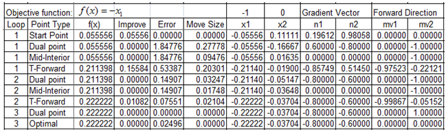
Table 3 lists step-by-step results for T-forward method to solve LP Example-1 with objective  .
.Table 3. T-forward method takes 2 forward steps to give exact optimal solution for LP Example-1. (objective
 ) )
 |
| |
|
Figure 6. also shows the first few T-forward steps for the results listed in Table 2 and Table 3. T-forward method takes only two forward steps to solve LP Example-1 and give exact optimal solution.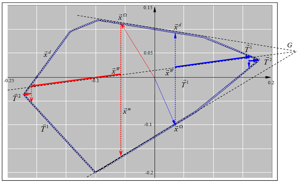 | Figure 6. Finding optimal solutions for LP Example-1 through T-forward method. The blue lines on the right side illustrate the T-forward path for maximizing  (see Table 2). The red lines on the left side illustrate the T-forward path for maximizing (see Table 2). The red lines on the left side illustrate the T-forward path for maximizing  (see Table 3). The vertical dashed lines represent the dual directions. T-forward method takes 2 forward steps to find exact optimal solution for both objective functions (see Table 3). The vertical dashed lines represent the dual directions. T-forward method takes 2 forward steps to find exact optimal solution for both objective functions |
15.2. Example 2: An LP with 2 Variables and 11 Constraints
Our second example is an LP problem that is used to describe the interior-point method at the website: http://en.wikipedia.org/wiki/Karmarkar's_algorithm. This problem can be formulated as: | (83) |
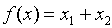
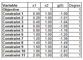
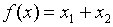
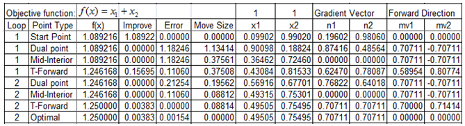
Table 4 lists the input data in table format for LP Example-2. Figure 7. shows the feasible boundary of this problem. By applying Equation (41), we can draw the feasible boundary  as shown in Figure 8. It can be observed that the boundary curve drawn through our closed-form Equation (41) is exactly the same as the feasible boundary as shown in Figure 7. This gives another validation for our closed-form solution. Table 5 lists step-by-step results for T-forward method to solve LP Example-2 with objective
  . T-forward method takes 2 forward steps to give exact optimal solution for this problem as shown in Figure 8., while interior method takes many steps to reach an ɛ-approximated solution as shown in Figure 7.
 Table 4. Input data for LP Example-2 with objective
 |
| |
|
 | Figure 7. The feasible boundary curve for LP Example-2. The red line represents the path searched by the interior method. This figure is used to describe the interior point method at the website http://en.wikipedia.org/wiki/Karmarkar's_algorithm |
Table 5. T-forward method gives exact optimal solution in 2 forward steps for LP Example-2 (objective
 ) )
 |
| |
|
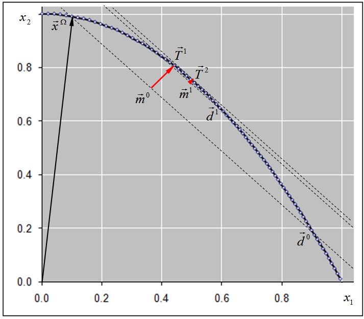 | Figure 8. Starting from a feasible boundary point  , T-forward method takes two steps to find the exact optimal solution for LP Example-2. The red arrow line represents the T-forward move. The dashed lines represent the dual direction , T-forward method takes two steps to find the exact optimal solution for LP Example-2. The red arrow line represents the T-forward move. The dashed lines represent the dual direction |
16. Complexity Analysis
Let us analyze the complexity for the T-forward-point method and the Facet-forward method introduced in previous sections.The T-forward-point method is simply to call the T-forward-function  repeatedly. Each T-forward-function
  , as shown in Equation (56), includes two calls of the boundary function
  and two calls of the gradient function
  . Each of these functions needs to calculate the roots
  for
for 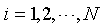 . The complexity for calculating one
  through Equation (67) is
  , where
  represents the maximum arithmetic calculations for calculating one
  or the length of the input for one constraint. For LP problems,
  . The complexity for calculating all the roots
  for
for 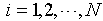 is
is  . Once
  is calculated, the boundary function
  and the gradient function
  can be calculated in
  . Thus, the T-forward-function
  can be calculated in
  . Now let us estimate how many T-forward steps are needed to find the optimal solution through T-forward method. Here we only consider convex NLP, which means the feasible region
  is convex.
 | Figure 9. Initially the residual feasible region is  , the residual feasible region is , the residual feasible region is  with with  as their upper bound ellipsoid. After one T-forward move, the residual feasible region becomes as their upper bound ellipsoid. After one T-forward move, the residual feasible region becomes  with with  as their upper bound ellipsoid. as their upper bound ellipsoid.  is an ellipsoid contained in is an ellipsoid contained in  and centered at and centered at  and an upper bound for and an upper bound for  . The curve . The curve  bisects the region AGDCA. The volume of bisects the region AGDCA. The volume of  is less than half of is less than half of  , and the volume of , and the volume of  is less than half of is less than half of  . Then, after one T-forward step, the residual feasible region is reduced at least be a factor of 4 . Then, after one T-forward step, the residual feasible region is reduced at least be a factor of 4 |
As illustrated in Figure 9. , at the initial feasible point  , we use the objective contour plane
  to cut the feasible region
  . The residual feasible region must be in the region bounded by the two plane curves
  and
and  , where
  is the tangent plane curve of
  passing the point
  , and
, and  is the tangent plane curve of
  passing through the dual point
  . Point G represents the common edge of the two plane curves
  and
and  . The line
  represents the bisector of the two curves
  and
and  . Before we start the T-Forward step, the upper bound ellipsoid of the residual feasible region is in the region GAD. Here we only consider the ellipsoid that is cut by the contour plane
  . After the first T-forward step, the feasible region is cut at the T-forward point
  . Since
  is designed to be along the direction
  , and it is a boundary point of the feasible region. Then the residual region after
  becomes the region
  , with
  as one of its boundary point. Thus
  must be either in the region GBT1 or GET1, either one is half of the region GBE. We draw another ellipsoid
  , which with
  as its center and upper bounded by
  , and with
  to be contained in
  . We should have:
 | (84) |
Therefore, each T-forward step moves the cutting plane  close to the target further and reduces the volume of the residual feasible region at least by a factor of 4. After K times of T-forward steps, the volume of the residual feasible region will be reduced by
  . The relative difference between the T-forward solution
  and the optimal solution
  will be reduced to the order of
  . In other words, if the requested precision is
  , we need to call T-forward function
  times.Ellipsoid method is proven to be polynomial through similar method as we used above [10, 11].In summary, the running time for T-forward method to give an
  -approximated solution for NLP is
  . If the problem is LP, the T-forward method can give exact optimal solution with complexity
  .The facet-forward method simply calls
  and
and  at most N times to give local optimal solution in a facet. It takes
  time to get a solution for one facet and have the number of constraint reduced at least by 1. Then, it needs to run at most N times to reduce all constraints and give final optimal solution for LP problems. Therefore, the running time for facet-forward method is
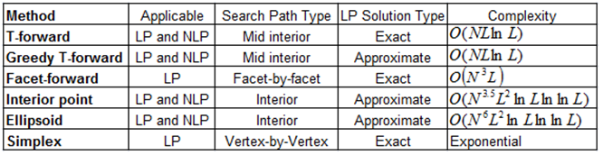
  . Table 6 compares the methods proposed in this paper with the current best known existing LP algorithms, including simplex method, the ellipsoid method, and the interior point method.
 Table 6. Comparison of the T-forward method with simplex, ellipsoid, and the interior point method
 |
| |
|
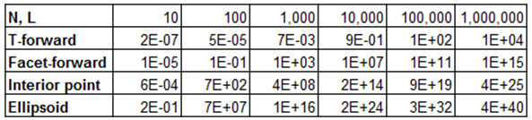
Suppose we run a computer with 1Ghz processor, Table 7 lists the estimated running time in seconds for various methods and various  and
and  . For simplicity, here we assume
  .
. Table 6. Estimated running time (in seconds) on a computer with 1 GHz processor
 |
| |
|
For example, if we want to solve an LP with  , our proposed T-forward method will take couple of seconds to solve it, while the interior point method will take
  years to solve the same problem, which is a mission impossible for most of the current existing LP algorithms.
17. Conclusions
The main contributions of this paper include the closed-form solutions for LP, QCQP, and the near-closed-form solution for NLP. Another contribution is the T-forward method for NLP and the facet-forward method for LP. Both methods are polynomial time. The T-forward method and the facet-forward method are not only faster than any existing LP or NLP algorithms, but also give exact optimal solution when applied to LP.
References
| [1] | [AG93] E. L. Allgower and K. Georg. “Continuation and path following”. Acta Numerica, 1993, Cambridge University Press, Cambridge, UK, 1993, pp. 1–64. |
| [2] | [AG97] E. L. Allgower and K. Georg. “Numerical path following”. Handbook of Numerical Analysis, Vol. 5, P. G. Ciarlet and J. L. Lions, eds., North-Holland, Amsterdam, 1997, pp. 3–207. |
| [3] | [AGJ00] P. Armand, J. C. Gilbert, and S. Jan-J´egou. “A feasible BFGS interior point algorithm for solving convex minimization problems”. SIAM J. Optim., 11 (2000), pp. 199–222. |
| [4] | [Bam86] E.R. Barnes. “A variation on Karmarkar’s algorithm for solving linear programming problems”. Mathematical Programming, 36:174–182, 1986. |
| [5] | [CSE00] Computing in Science and Engineering, volume 2, no. 1, 2000. |
| [6] | [CO00] A. R. Conn, N. I. M. Gould, D. Orban, and P. L. Toint. “A primal-dual trust-region algorithm for non-convex nonlinear programming”. Math. Program., 87 (2000), pp. 215–249. |
| [7] | [CG97] A. R. Conn, N. I. M. Gould, and P. L. Toint. “A globally convergent Lagrangian barrier algorithm for optimization with general inequality constraints and simple bounds”. Math. Comp., 66 (1997), pp. 261–288, S1–S11. |
| [8] | [FG98] A. Forsgren and P. E. Gill. “Primal-dual interior methods for nonconvex nonlinear programming”. SIAM J. Optim., 8 (1998), pp. 1132–1152. |
| [9] | [Kar84] N. K. Karmarkar. “A new polynomial-time algorithm for linear programming”. Combinatorica, 4:373–395, 1984. |
| [10] | [Kha79] L. G. Khachiyan, “A Polynomial Algorithm in Linear Programming”. Doklady Akademii Nauk SSSR 244:S (1979), 1093-1096, translated in Soviet Mathematics - Doklady 20:1 (1979), 191-194. |
| [11] | [KK79] Kozlov, M. K.; S. P. Tarasov and Leonid G. Khachiyan (1979). “Polynomial solvability of convex quadratic programming”. Doklady Akademii Nauk SSSR 248: 1049–1051, translated in Soviet Mathematics - Doklady 20: 1108–1111 |
| [12] | [KM72] V. Klee, G. Minty. “How good is the simplex algorithm?” Inequalities III, New York-London: Academic Press: pp. 159-175. |
| [13] | [Meh92] Mehrotra, Sanjay. "On the Implementation of a Primal-Dual Interior Point Method". SIAM Journal on Optimization 2 (4): 575, 1992. |
| [14] | [MW01] G. P. McCormick and C. Witzgall. “Logarithmic SUMT limits in convex programming”. Math. Program., 90 (2001), pp. 113–145. |
| [15] | [Pol92] R. Polyak. “Modified barrier functions (theory and methods)”. Math. Program., 54 (1992), pp. 177–222. |
| [16] | [VM86] R. J. Vanderbei, M. S. Meketon, and B. A. Freedman. “A modification of Karmarkar’s linear programming algorithm”. Algorithmica, 1:395–407, 1986. |
| [17] | [Wri04] M. H. Wright, “The interior-point revolution in optimization: History, recent developments, and lasting consequences”. Bulletin of the American Mathematical Society 42: 39, 2004. |
 Abstract
 Reference
 Full-Text PDF
 Full-text HTML