1. Introduction

We find the solution of an ill conditioned linear system by transforming it using the additive preconditioning and the Schur aggregation. We use the Sherman-Morrison-Woodbury (SMW) formula where is an invertible square matrix and to get new linear systems. The challenge in solving these new linear systems of smaller sizes with well conditioned coefficients matrices , and is the computation of the Schur aggregate S. The technique of (extended) iterative refinement or improvement for computing the Schur aggregate[14] and its application for solving linear systems of equations has been studied in a number of papers[3, 15, 18]. Its variant that we used allows us to compute with high precision. The high precision is achieved by minimizing the errors in the computation. The bound of the forward error will allow us to determine if the computed solution is an accurate one. This paper is divided into three sections. The first section covers the concept of rounding errors, floating-point summation, matrix norms and convergence. The second section is devoted to the additive preconditioning, the Schur aggregation and how the iterative refinement or improvement technique is used with the SMW formula to transform the original linear system into better conditioned linear systems. The third section analyzes the forward error of the extended iterative refinement or improvement algorithm and provides a forward error bound.

2. Rounding Errors, Floating-point Summation, Matrix Norms and Convergence

2.1. Rounding Errors

Definition 2.1.1 Let be an approximation of the scalar x. The absolute error in approximatingis the number .

Definition 2.1.2 Let be an approximation of a scalar . The absolute and relative errors of this approximation are the numbers and , respectively. If is an approximation to with relative error, then there is a number such that 1) and 2) .

Remark 2.1.1 The relative error is independent of scaling, that is the scalingand leave unchanged.

Theorem 2.1[6] Assume that approximates with relative error < 1.

Then is nonzero and.

Remark 2.1.2 If the relative error of with respect to is , then and agree to roughly correct significant digits. For binary system, if and have relative error of approximately , then and agree to about bits.

Definition 2.1.3 The componentwise relative error is defined as: for and is widely used in the error analysis and perturbation theory.

Remark 2.1.3 In numerical computation, one has three main sources of errors.

1. Rounding errors, which are unavoidable consequences of working in finite precision arithmetic.

2. Uncertainty in the input data, which is always a possibility when we are solving practical problems.

3. Truncation errors, which are constituted and introduced by omitted terms.

Rounding errors and Truncation errors are closely related to forward errors.

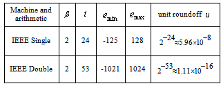
Definition 2.1.4 Precision is the number of digits in the representation of a real number. It defines the accuracy with which the computations and in particular the basic arithmetic operations are performed. For floating point arithmetic, precision is measured by the unit roundoff or machine precision, which we denote u in single precision and ū in double precision. The values of the unit roundoff are given in Table 1.1 in Section 2.3.

Remark 2.1.4 Accuracy refers to the absolute or relative error of an approximation.

Definition 2.1.5 Let be an approximation of computed with a precision where is a real function of a real scalar variable.

is called the (absolute) backward error, whereas the absolute or relative errors of are called forward errors.

Definition 2.1.6 For an approximation to a solution of a linear system with and , the forward error is the ratio .

The process of bounding the forward error of a computed solution in terms of is called forward error analysis. is the perturbation of .

Definition 2.1.7 An algorithm is called forward stable if it produces answers with forward errors of similar magnitude to those produced by backward stable method.

Definition 2.1.8 A mixed forward-backward error is defined by the equation

where , withand are small constants.

Remark 2.1.5 This definition implies that the computed value ŷ differs little from the value that would have been produced by an input little different from the actual input . Simpler, is almost the right answer for almost the right data.

Definition 2.1.9 An algorithm is called numerically stable if it is stable in the mixed forward and backward error sense.

Remark 2.1.6 A backward stability implies a forward stability but the converse is not true.

Remark 2.1.7 One may use the following rule of thumb;

Forward error condition numberbackward error, with approximate equality possible. Therefore the computed solution to an ill conditioned problem can have a large forward error even if the computed solution has a small backward error. This error can be amplified by the condition number in the transition to forward error. This is one of our motivations for reducing the condition number of the matrix A using the additive preconditioning method.

Definition 2.1.10 For a system of linear equations , is called the relative residual. The relative residual gives us an indication on how closely represents and is scale independent.

2.2. Floating-point Number System

Definition 2.2.1[6] A floating-point number system is a subset of the real numbers whose elements have the form. The range of the nonzero floating-point numbers in is given by . Any floating-point number can be written in the form where each digit satisfies and for normalized numbers. is called the most significant digit and the least significant digit.

2.3. Error-free Floating-point Summation

Here is a summation algorithm due to D.E. Knuth[7]. Algorithm 1. Error-free transformation of the sum of two floating point numbers

The algorithm transforms two input-floating point numbers and into two output floating-point numbers and such that and . The same solution is achieved using the Kahan-Babušhka’s[11] and Dekker’s[12] classical algorithm provided that . It uses fewer ops but includes branches, which slows down the code optimization outputs.

Definition 2.3.1[8] The unit roundoff error is the quantity . We write and to denote the operations performed in single precision and in double precision, respectively.

Table 1.1. The values of the unit roundoff

Remark 2.3.1 The following theorem shows that every real number lying in can be approximated by an element of with a relative error no larger than .

Theorem 2.2 Iflies in then with <

Theorem 2.2 says that is equal to multiplied by a factor very close to 1.

Definition 2.3.2 From now on , for an argument that is an arithmetic expression, denotes the computed value of that expression. op represents floating-point operation in .

2.4. Matrix Norms

2.4.1. The Singular Value Decomposition (SVD)[3, 15]

Definition 2.4.1 The compact singular value decomposition or SVD of an matrix of a rank is the decomposition: where and are unitary matrices, that is, ,,is a diagonal matrix, and are m- and n-dimensional vectors, respectively, and > 0. or for is the largest singular value of the matrix .

Definition 2.4.2 The condition number, of a matrix of a rank is . A matrix is said to be ill conditioned if its condition number is large, that is if , and is called well conditioned otherwise.

Definition 2.4.3[6] The matrix 2-norm

= = , is also called the spectral norm. denotes the largest singular value of the matrix .

Remark 2.4.1 The matrix 2-norm satisfies the relation

1. where

, for and.

2. .

Lemma 2.3 For a vector norm , suppose that

< 1 . Then .

2.5. Numerical Nullity

Definition 2.5.1 The nullity of , , is the smallest integer for which a rank APC can define a nonsingular A-modification . The nullity of , which is defined as the dimension of the null space can also be defined as the large integer r for which we have or , provided is a nonsingular matrix. In this case, and are the right and left null matrix bases for the matrix A.

Definition 2.5.2 The numerical nullity of is the number of its small singular values.

2.6. Convergence

There is a natural way to extend the notion of limit from to .

Definition 2.6.1 Let be a sequence of vectors in and let . The sequence converges componentwise to and we write

if for .

Here is another way to define convergence in .

Definition 2.6.2 Let be a sequence of vectors in and let . The sequence converges normwise to , that is

if and only if

There is no compelling reason to expect the two notions of convergence to be equivalent. In fact for infinite dimensional vector space, they are not.

Theorem 2.4[6] Let and suppose that .

Then is nonsingular and (this sum is called Neumann sum). A sufficient condition for is that < 1 in some consistent norm, in which case .

Corollary 2.5 If , then is nonnegative and .

Theorem 2.6[6] Let be a matrix norm on

consistent with a vector norm (also denoted) and let a matrix . Let be a square matrix such that

< 1. Then

(i) the matrix is nonsingular,

(ii) , and

(iii) .

The following corollary extends Theorem 2.6.

Corollary 2.7[6]

If , then .

Moreover, ,

so that .

The corollary remains valid if all occurrences of are replaced by .

Theorem 2.8 [8, 17] Let denote a matrix norm and a consistent vector norm. If the matrix is nonsingular and and (i) , where is an approximated value of x, then

(ii) .

In addition if < 1, then is nonsingular and

(iii) .

3. The Additive Preconditioning Method, the Schur Aggregation and the Extended Iterative Refinement or Improvement Algorithm

3.1. The Additive Preconditioning Method

Definition 3.1.1 For a pair of matrices of size and of size , both having full rank r > 0, the matrix of rank r is an additive preprocessor (APP) of rank r for any matrix. The matrixis the A-modification. The matrices and are the generators of the APP, and the transition is an A-preprocessing of rank r for the matrix . An APP for a matrix A is an additive preconditioning (APC) and an A-preprocessing is an A-preconditioning if . An APP is an additive compressor (AC) and an A-preprocessing is an A-complementation if the matrix A is rank deficient, whereas the A-modification C has full rank. An APP is unitary if the matrices and are unitary.

Remark 3.1.1 Suppose has rank r. Then[3, 18], we expect to be to the order of , therefore small if the additive preconditioner is

i) random

ii) well conditioned, and

iii) properly scaled, that is is not large and not small.

Additive preconditioning consists in adding a matrix of a small rank to the input matrix , to decrease its condition number. The A-modification is supposed to generate a well conditioned matrix. In practice, to compute the A-modification error-free, we fill the generators and with short binary numbers.

3.2. The Schur Aggregation

The aggregation method consists of transforming an original linear system into linear systems of smaller sizes with well conditioned coefficients matrices , , and . The aggregation method is a well known technique[3, 14, 15, 18], but aggregation used here both decreases the size of the input matrix and improves its conditioning. One may remark that aggregation can be applied recursively until no ill conditioned matrix appears in the computation.

Definition 3.2.1 The Schur aggregation is the process of reducing the linear system by using the SMW (Sherman-Morrison-Woodbury) formula

. The matrix, which is the Schur complement (Gauss transform) of the blockin the block matrix , is called the Schur aggregate. The A-modification and the Schur aggregate are well conditioned, therefore the numerical problems in the inversion of the matrix A are confined to the computation of the Schur aggregate .

3.3. The Iterative Refinement or Improvement Algorithm

Let . Then, we apply the Sherman-Morrison -Woodbury (SMW) formula to the original linear system and transform it into better conditioned linear systems of small sizes, with well conditioned matrices , and . We solve the original linear system by post-multiplying by the vector b. We consider the case where the matrices C and S are well conditioned, whereas the matrices and have small rank r, so that we can solve the above linear systems with the matrices and faster and more accurately than the system with the matrix . In this case the original conditioning problems for a linear system are restricted to the computation of the Schur aggregate .

To compute the Schur aggregatewith precision, we begin with computing using the iterative refinement or improvement algorithm. We prove that we can get very close to the solution W of the linear system . We closely approximate it by working with numbers rounded to the IEEE standard double precision and using error-free summation. All norms used in this section are the 2-norm. The iterative refinement or improvement algorithm is a technique for improving the computed approximate solution of a linear system . Iterative refinement or improvement for the Gaussian Elimination (GE) was used in the 1940s on desk calculators, but the first thorough analysis of the method was given by Wilkinson in 1963. The process consists of three steps ([6],[7],[15]).

Algorithm 2. Basic iterative refinement or improvement algorithm

Input: An matrix, a computed solution to and a vector b.

Output: A solution vector approximating in and an error bound .

Initialize:

Computations:

1) Compute the residual in double precision ()

2) Solve in single precision (u) using the GEPP

3) Update in double precision ()

Repeat stages 1-3 until is accurate enough.

Output and an error bound.

The iterative refinement or improvement algorithm can be rewritten as follows[6]. is the error in the computation of , is the error in the computation of and , where is the perturbation to the matrix A. is a computed solution of the linear system .

1)

2)

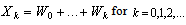
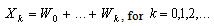
3)

Repeat stages 1-3.

The algorithm yields a sequence of approximate solutions which converges to .

We use the extension of Wilkinson’s iterative refinement or improvement to compute the matrix with extended precision. In its classical form, above the algorithm is applied to a single system , where and are vectors. We applied it to the matrix equation , where the solution we are seeking is the matrix . In its classical version, also the refinement stops when the matrix is computed with at most double precision. In order to achieve the high precision in computing W, we apply a variant of the extended iterative refinement or improvement where the residuals dynamically decrease, which is a must for us. We represent the output value as the sum of matrices with fixed-precision numbers.

3.4. The Extended Iterative Refinement or Improvement

Suppose is an ill conditioned non-singular matrix with where is the numerical nullity of the matrix , is a random, well conditioned and properly scaled APC of rank r < n, and the well conditioned A-modification . We use the matrices and whose entries can be rounded to a fixed (small) number of bits to control or avoid rounding errors in computing the matrix .

Surely, small norm perturbations of the generators and , caused by truncation of their entrees, keep the matrix C well conditioned. We rewrite the iterative refinement or improvement algorithm to solve the linear system with and as follows.

Algorithm 3.

(0.1)

(0.2)

(0.3)

The solution W of the linear system is computed by means of Gaussian Elimination with Partial Pivoting (hereafter GEPP), which is a backward stable process. It is corrupted by rounding errors of the computation of in (0.1), so that the computed matrix (computed in single precision arithmetic u) turns into . is the perturbation to the matrix C. We can also say equivalently that there exists an error matrix such that

(0.4)

that is, is an exact solution for the approximated problem. is a constant function of order . Another source of error is the computation in (0.2) which, done using double precision arithmetic , turns numerically into

(0.5)

where

(0.6)

(0.7)

We recall that the summation (0.3) is done error free.

Algorithm 4. Let us solve the linear system , derived from the ill conditioned linear system , by applying the following extended iterative refinement or improvement algorithm.

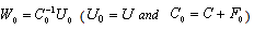
(0.8)

(0.9)

Let .

Theorem 3.1[1]

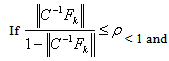(0.10)

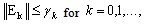(0.11)

then In other words, is bounded by for a certain integer k.

Proposition 3.2 Let be nonsingular and let consider the linear system. If <ρ < 1, then the matrix is nonsingular and

where

(0.12)

or equivalently,

.

4. Forward Error Analysis

Our forward error analysis of the extended iterative refinement or improvement algorithm results with the following proposition.

Proposition 4.1 (Forward error bound) Let be a linear system derived from an ill conditioned linear system where is , is both with full rank r> 0, and is a well conditioned A-modification. If is solved using the extended iterative refinement or improvement algorithm, Algorithm (4.) then for sufficiently large the forward error is bounded by . That is

where and are constant functions of order k. Furthermore we have

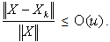The forward error is bounded by a constant in the order of u which is an important result.

Proof: We obtain from equation (0.4),

.

Since , we get

by using (0.4).

by using (0.5),

by using (0.12) in Proposition (3.2),

,

by using (0.2).

We have,

,

,

, so that

,

Consequently

, so

.

Without loss of generality we can assume that .

Recall that < 1, and take the norm on both sides, to get

.

Recalling (0.6) and (0.7), we deduce that

We recall the following inequalities (0.12),

< 1.

From (0.7) ,

Therefore ,

.

So .

We recall (0.6) .

We also have

where

and

.

and are constant functions of order .

< 1 and < 1 since C is well conditioned, we deduce that

.

Therefore, .

We also recall that

,

so that

and …

. Therefore,

.

Therefore for sufficiently largek, we have

. Moreover,

. So,

where and are constant functions of order . Therefore, .

5. Conclusions

We use the concepts of additive preconditioning and Schur aggregation along with the extended iterative refinement or improvement algorithm to reduce the computation of to the computation of the Schur aggregate . We solve the linear system with high precision using the extended iterative refinement or improvement algorithm. We proved in our forward error analysis that the forward error is bounded by . The forward error can further be bounded by , a constant of order u. These results are in line with Higham’s results ([6], page 234, Theorem 11.1) and constitute another way to prove the convergence of the extended iterative refinement or improvement to a more accurate solution

.

ACKNOWLEDGEMENTS

The author would like to thank Professor Victor Pan, Distinguished professor of The City University of New York for his support and advice. The author would also like to thank his wife Lisa C. Serme for her support.