1. Introduction

In any environment, the main objective is to provide a set of best alternatives for given criteria. The decision maker provides some necessary and basic information about each criterion and the alternatives that helps in identifying the relation between them. The problems of this kind can be dealt with Multi Criteria Decision Making or Multi Criteria Decision Aid (MCDA) techniques.

The main aim of MCDA is to account for several views and provide some tools for the Decision Maker (DM) in solving complex decision problems. The trade-off between the criteria and DM’s preferences lies in providing compromise solutions. In each and every problem or situation, the DM, Stakeholder and Analyst play an important role.

DM is a person, who has a great impact in evaluating the situation, expressing preferences, considering solutions and approving the final result. Stakeholders are members involved in decision situation and interested in finding a solution for the problem. For the situation considered, the Analyst is responsible in recognizing the consequences and selecting an appropriate decision aiding method/tool for the construction of decision models.

In every MCDA problem environment, each criterion will be embedded with a set of alternatives out of which one alternative will act as the best for that particular criterion. These set of alternatives will be finite if a proper definition about all the members is given, otherwise infinite. If the number and content of alternatives are fixed and cannot be varied during the decision aiding process, then this nature is said to be stable otherwise volatile. At the final stage of the decision aiding process, if we come across a single best alternative which excludes the possibility of choosing any other alternative, it is referred as Comprehensive and if we opt for a combination of alternatives, it is fragmented. . In brief, the alternatives are estimated on a set of criteria. The criterion defines the feature and some properties of the set of alternatives.

Notations

x_i : i^th alternative (i=1,…,m)

X : Set of alternatives

g_j : jth criterion (j=1,…,n)

G : set of criteria

Q_j : jth Indifference thresholds

P_j : jth Preference thresholds

W_j : jth Weights

V_j : jth Veto thresholds

λ : Cutting level

b_q : q^th boundary alternative (q = 1,…,s)

B : set of boundary alternatives (b₁, b₂, …, b_q)

l_q : q^th boundary class

C_j (x_i, b_q) and D_j (x_i, b_q) : partial concordance and partial discordance of the x_i and b_q

C_j (b_q, x_i) and D_j (b_q, x_i) : partial concordance and partial discordance of the b_q and x_i

C (x_i, b_q) and C (b_q, x_i) : overall concordance indices

S_j (x_i, b_q): outranking index for x_i and b_q

S_j (b_q, x_i): outranking index for b_q and x_i

C_q : q^th category

P : strict preference

Q : weak preference

I : indifference

J : incomparability

The entire MCDA problem will be expressed in terms of relations existing between the alternatives and criteria. We brief out each and every relation and the nomenclature for it.

1.1. Relations

• The indifference relation between two alternatives x_i and x_r, denoted as x_iIx_r, means that the two alternatives x_i and x_r are equally preferable or equally important to the DM. This relation is reflexive and symmetric.

• The strict preference is a relation of x_i over x_r, denoted as x_iPx_r, which gives the meaning that x_i is better than the x_r for the DM. It is asymmetric and non-reflexive.

• The weak preference is a relation which hesitates to make a specific judgment about the preference or indifference between x_i and x_r, denoted by x_iQx_r. It is also asymmetric and non-reflexive.

• If x_i is not in any of the above mentioned relations with x_r, then it is referred to as incomparability relation, denoted by x_iJx_r. This relation is symmetric and non-reflexive.

• The outranking relation is denoted as x_iSx_r. It defines the situation in which the preference (strong- x_iPx_r or weak- x_iQx_r) or indifference relation (x_iIx_r) is true or not.

In order to observe a specific type of relation between alternative and criterion, there is a need to compute some indices such as partial concordance, discordance and outranking indices. over the years, many methodologies were developed of which the most familiar method is the Outranking Methodology. In outranking methodology, we have considered ELECTRE TRI method and for this we have developed spreadsheet algorithms, which support the analyst to analyze and to provide a better decision making. First we review some literature confining to ELECTRE TRI method and then a detailed algorithmic approach is given along with the results.

2. Outranking Methodology

In MCDA, the outranking methodology comes under the framework of classification problems. Basing on the same criterion, the methodology allows comparing the pairs of alternatives by considering indifference, preference and veto thresholds. This helps in determining the indifference, preference to one over the other and incomparable relation between alternatives. The seminal work on this methodology was proposed by B. Roy (1965). He developed some mathematical structures about the ELECTRE family which help in choosing the best alternative from the set of alternatives. In recent years, many state of art surveys were conducted and reported on the development of the MCDA methodologies by M.Bruen and L. Maystre (2000), B.Roy and J. Figueira (2002), J. Martel and B. Matarezzo (2005), J. Figueira, V. Mousseau and B.Roy (2005).

B. Roy (1977, 1981) proposed the Trichotomic segmentation outranking based classification method for sorting problems with three classes. Later, this method was extended to an arbitrary number of classes in N-TOMIC by R. Massagliaet (1991) and few ELECTRE methods by V. Mousseau et al (1998) and W. Yu (1992).

2.1. ELECTRE TRI Method

ELECTRE method helps to identify the outranking relations between pairs of alternatives for each criterion. In classification problems, a given set of alternatives X with a set of criteria G are to be assigned into a set of ordered classes L by the predefined set of boundary alternatives B. Each class is considered by two (upper and lower) boundary alternatives. The upper bound b_q of the class l_q-1 is the lower bound of the class l_q (q=1,…,s). Changing the least one criterion moves the boundary alternative to the neighbouring class.

For solving the classification problem the method estimates the outranking relation for each alternative x_i ϵ X (i=1,…,m) which is to be classified and each boundary alternative b_q between classes l_q-1 and l_q by calculating the outranking index. If l_q is preferred to the lower boundary alternative l_q-1 of the class, we assign the alternative x_i to the class l_q and the upper boundary alternative b_q of the class is preferred to this alternative.

For calculating the outranking index, the DM should give the information about

(i) the set of alternatives to be classified

(ii) the set of criteria on which alternatives are evaluated with a scale of quantitative values for each criterion.

(iii) the number of classes as well as their order according to preference.

(iv) the upper and lower boundary alternatives for each class l_q

For each criterion g_j (j=1,…,n), the ELECTRE TRI method requires to define the preference p_j(^.), indifference q_j(^.), veto v_j(^.) thresholds as well as weights w_j and cutting level λ (should lie between 0.5 and 1).

(a) the preference p_j(^.) threshold indicates the smallest difference between two alternatives on the criterion g_j, that is one alternative is preferred to the other.

(b) the indifference q_j(^.) threshold indicates the largest difference between two alternatives on the criterion g_j.

(c) the veto v_j(^.) threshold indicates the smallest difference between the alternatives on the criterion g_j, that says incomparability of these two alternatives.

(d) All the above three thresholds should satisfy the constraint, v_j (^.) > p_j (^.) > q_j (^.)

(e) the weight w_j indicates the relative importance of criterion when compare to the other criterion in terms of votes.

(f) the cutting level λ shows the smallest value of the outranking index, which is sufficient for considering an outranking situation between two alternatives.

The outranking relation is verified by two conditions; concordance and discordance, with respect to the thresholds, weights and cutting level λ. Concordance requires preference of the alternative x_i over the boundary alternative b_q on the majority of criteria. Discordance demands the absence of strong opposition to the first condition in the majority of criteria. We need to compute two partial indices for each criterion, that is partial concordance C_j (x_i, b_q) and C_j (b_q, x_i) and partial discordance D_j (x_i, b_q) and D_j (b_q, x_i). The above partial indices help in computing the outranking indices S_j (x_i, b_q) and S_j (b_q, x_i). Using a specific cutting level λ, a comparison of outranking indices is possible and turns to two types of assignment procedures namely pessimistic and optimistic.

The pessimistic procedure starts with the comparison of an alternative to the lower bound of the highest class and the optimistic procedure starts with the comparison of an alternative to the upper bound to the lowest class. In section 3, we describe the mathematical structures of outranking indices and assignment procedures.

3. Algorithm of the ELECTRE TRI Method

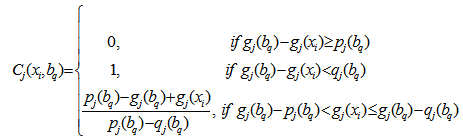
The ELECTRE TRI method has been divided into two parts; part I is to compute the outranking indices and to identify the relations between the alternatives and criteria and in part II, using the obtained outranking relation and cutting level λ, we provide the final result for the MCDA problem.

Part I: To construct the outranking relation x_i S b_q for each alternative x_i to be classified and each boundary alternative b_q.

1. Calculate the partial concordance indices C_j (x_i, b_q) and C_j (b_q, x_i) for each criteria g_j according to the increasing direction of preferences. The partial concordance index C_j (x_i, b_q) is as follows

The partial concordance index C_j (b_q, x_i) is as follows

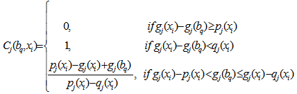2. To find the overall concordance indices C (x_i, b_q) and C (b_q, x_i) as an aggregation of partial concordance indices.

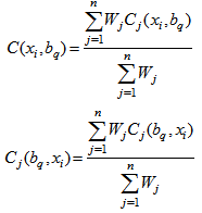3. Calculate partial discordance indices D_j (x_i, b_q) and D_j (b_q, x_i) for each criteria g_j. We compute the partial discordance index D_j (x_i, b_q) according to the increasing direction of preference.

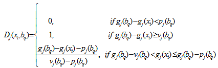The partial discordance index D_j (x_i, b_q) is as follows

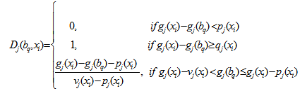4. Calculate the outranking indices S(x_i, b_q) and S(b_q, x_i), that shows outranking creditability. The creditability index of x_i over b_q assuming S(x_i, b_q) ϵ[0,1] as follows

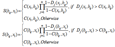5. The value of outranking indices is compared to the cutting level , which is defined by the DM and lies in the interval[0.5, 1].

• If S(x_i, b_q) ≥ and S(b_q, x_i) ≥ x_iIb_q, then the alternative x_i and b_q are indifferent.

• If S(x_i, b_q) ≥ and S(b_q, x_i) < x_iPb_q or x_iQb_q, then the alternative x_i is strongly or weakly preferred to the boundary alternative b_q.

• If S(x_i, b_q) < and S(b_q, x_i) ≥ b_qPx_i or b_qQx_i, then the boundary alternative b_q is strongly or weakly to x_i.

• If S(x_i, b_q) < and S(b_q, x_i) < x_iJb_q, then the alternative x_i and b_q are incomparable.

Part II:

On using the computed outranking indices in Part I, the DM has an option to choose either an optimistic procedure or a pessimistic procedure or both. After choosing an alternative procedure, the comparison of outranking indices for each pair of alternative x_i will be classified using each boundary alternative to the cutting level .

3.1. The Pessimistic Procedure

In this procedure the comparison will start from alternative x_i to the lower bound b_q-1 of the highest class l_q (q=s,…,1) and continues in decreasing order until, a lower bound b_q-1 is found, that is x_iSb_q-1, and for estimating the outranking relation we calculate S(x_i , b_q-1). Once the outranking relation is obtained, we calculate outranking index between x_i and b_q. We assign the alternative x_i to the l_q if S(x_i, b_q-1) ≥ and S(x_i, b_q) < .

1. Compare x_i successively to b_q for q= s,s-1,…,0

2. b_q being the first bound such that x_iSb_q, assign x_i to category C_q+1 (x_i →C_q+1)

In other words, the above procedure can also be expressed as follows; b_q-1 and b_q are upper and lower bound of category C_q, the pessimistic procedure assigns alternative x_i to the highest category C_q such that x_i Sb_q-1. When using this procedure with =1, an alternative x_i can be assign to category C_q only if g_j(x_i) equals or exceeds g_j(b_q-1) for each criterion. When decreases the pessimistic characters of this rule is weakened.

3.2. The Optimistic Procedure

Here, we begin to compare the alternative x_i to the upper bound b_q of the lowest class l_q (q=1,…,s) and proceed in increasing order until we find such a upper bound bq that has strict preferences over the alternatives x_i, then we calculate S(x_i, b_q-1) and assign that alternative to the class l_q if S(x_i, b_q-1) ≥ and S(x_i, b_q) <.

1. Compare x_i successively to b_q for q=1,…,s.

2. b_q being the first bound such that b_qPx_i, assign x_i to C_q (x_i →C_q)

The optimistic procedure assign to x_i to the lowest category C_q for which the upper bound b_q is preferred to x_i. When using this procedure with = 1, an alternative x_i can be assigned to category C_q when g_j(b_q) exceeds g_j(x_i) at least for one criterion. When decreases the optimistic character of this rule is weakened.

3.3. Comparison of Two Assignment Procedures

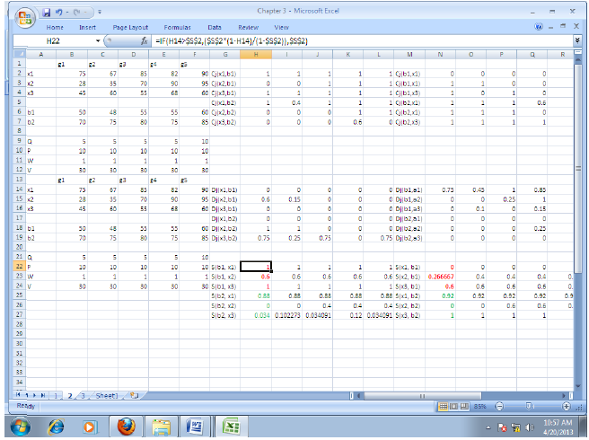
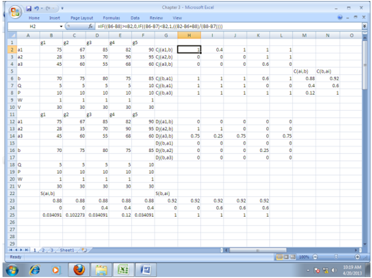
Let us suppose that an alternative x_i is assigned to C_q and C_r by the pessimistic and optimistic procedures, if the following conditions holds good

• C_q is lower or equal to C_r (q ≤ r)

• C_q > C_r, when x_iJb_F for every F, r ≤ F < q.

More specifically when the evaluation of an alternative are between the two boundary alternatives of a category on each criterion, then both procedures assign this alternative to this criterion. x_i divergence exists among the results of the two assignment procedures only when an alternative is incomparable to one or several b_q, in such case the pessimistic rule assigns the alternative to lower category than the optimistic.

Here, we demonstrate a spreadsheet algorithm for the ELECTRE TRI method using a numerical illustration. We have programmed two algorithms, of which the first one helps in finding the values of partial concordance and discordance along with the outranking index between x_i and b_q and the second algorithm provides solution for b_q and x_i.

Algorithm 3.1

Step 1: Enter the criteria values along with alternatives in ‘mxn’ design.

Step 2: Enter threshold values in a separate row below to the mxn design.

Step 3: To compute the partial concordance between i^th criteria and j^th alternative Cj(x_i, b_q) the following ‘NESTED IF ( )’ condition has been used

=IF ((B6-B10)>=B2, 0, IF ((B6-B9)Step 4: Repeat Step 3 for finding the left out concordance values.

Step 5: The overall concordance of two alternatives C(x_i, b_q) can be obtained using

‘SUMPRODUCT()’function =SUMPRODUCT (H2:L2,B11:F11)/SUM(B11:F11)

Step 6: To compute the partial discordance between i^th criteria and j^th alternative Dj(x_i, b_q), the following ‘NESTED IF ( )’ condition has been used

=IF((B20-B24)=B16,1,((B20-B16-B24)/(B26-B24))))

Step 7: To compute the out ranking index between i^th criteria and j^th alternative S(x_i, b_q) the following ‘IF ( )’ condition has been used

=IF(H16>$S$2,($S$2*(1-H16)/(1-$S$2)),$S$2)

Algorithm 3.2

Step 1: Enter the criteria values along with alternatives in ‘mxn’ design.

Step 2: Enter threshold values in a separate row below to the mxn design.

Step 3: To compute the partial concordance between i^th criteria and j^th alternative Cj(b_q , x_i) the following ‘NESTED IF ( )’ condition has been used

=IF((B6+B10)<=B2,0,IF((B6+B9)>B2,1,((B6-B2+B10)/(B10-B9))))

Step 4: Repeat Step 3 for finding the left out concordance values.

Step 5: The overall concordance of two alternatives

C(b_q , x_i) can be obtained using ‘SUMPRODUCT()’function =SUMPRODUCT(N2:R2,B11:F11)/SUM(B11:F11))

Step 6: To compute the partial discordance between i^th criteria and j^th alternative Dj(b_q , x_i), the following ‘NESTED IF ( )’ condition has been used

=IF((B16-B20)=B26,1,((B16-B20-B24)/(B26-B24))))

Step 7: To compute the out ranking index between i^th criteria and j^th alternative S(b_q , x_i) the following ‘IF ( )’ condition has been used

=IF(H16>$T$2,($T$2*(1-H16)/(1-$T$2)),$T$2)

4. Numerical Illustrations

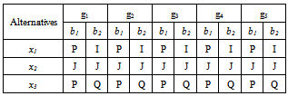
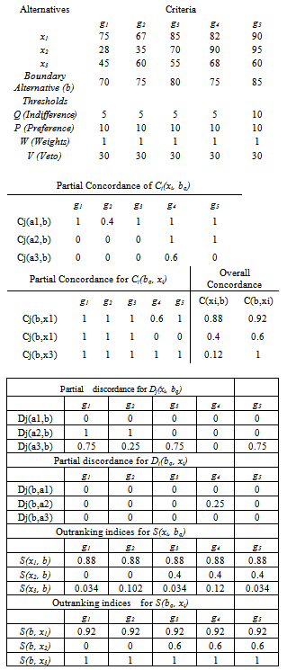
Let us consider an MCDA problem which has five criteria and three alternatives for each criterion. The table below gives the boundary alternatives b₁ and b₂ and various thresholds given by the decision maker (DM).

4.1. EXAMPLE 1

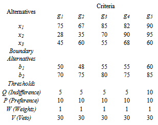Now, using the algorithm 3.1 and 3.2, the following values are computed. Along with the partial concordance and discordance, the overall concordance is also reported in the tables 1, 2, 3 and 4.

Table 1. Partial concordance of Cj(xi, bq) Partial Concordance of Cj(xi, bq) g1 g2 g3 g4 g5 Cj(x1,b1) 1 1 1 1 1 Cj(x2,b1) 0 0 1 1 1 Cj(x3,b1) 1 1 1 1 1 Cj(x1,b2) 1 0.4 1 1 1 Cj(x2,b2) 0 0 0 1 1 Cj(x3,b2) 0 0 0 0.6 0

Table 2. Partial concordance and overall concordance Partial Concordance for Cj(bq, xi) Overall Concordance g1 g2 g3 g4 g5 C(xi,b) C(b,xi) Cj(b1,x1) 0 0 0 0 0 1 0 Cj(b1,x1) 1 1 0 0 0 0.6 0.4 Cj(b1,x3) 1 0 1 0 1 1 0.6 Cj(b2,x1) 1 1 1 0.6 1 0.88 0.92 Cj(b2,x1) 1 1 1 0 0 0.4 0.6 Cj(b2,x3) 1 1 1 1 1 0.12 1

Table 3. Partial discordance for Dj(bq, xi) Partial discordance for Dj(bq, xi) g1 g2 g3 g4 g5 Dj(b1,x1) 0.75 0.45 1 0.85 1 Dj(b1,x2) 0 0 0.25 1 1 Dj(b1,x3) 0 0.1 0 0.15 0 Dj(b2,x1) 0 0 0 0 0 Dj(b2,x2) 0 0 0 0.25 0 Dj(b2,x3) 0 0 0 0 0

Table 4. Partial discordance for Dj(xi, bq) Partial discordance for Dj(xi, bq) g1 g2 g3 g4 g5 Dj(x1,b1) 0 0 0 0 0 Dj(x2,b1) 0.6 0.15 0 0 0 Dj(x3,b1) 0 0 0 0 0 Dj(x1,b2) 0 0 0 0 0 Dj(x2,b2) 1 1 0 0 0 Dj(x3,b2) 0.75 0.25 0.75 0 0.75

On the basis of the above four tables, we have calculated the outranking indices for both S(b_q, x_i) and S(x_i, b_q)

Table 5. Outranking indices for S(xi, bq) Outranking indices for S(xi, bq) g1 g2 g3 g4 g5 S(x1, b1) 0 0 0 0 0 S(x2, b1) 0.267 0.4 0.4 0.4 0.4 S(x3, b1) 0.6 0.6 0.6 0.6 0.6 S(x1, b2) 0.92 0.92 0.92 0.92 0.92 S(x2, b2) 0 0 0.6 0.6 0.6 S(x3, b2) 1 1 1 1 1

Table 6. Outranking indices for S(xi, bq) Outranking indices for S(bq, xi) g1 g2 g3 g4 g5 S(b1, x1) 1 1 1 1 1 S(b1, x2) 0.6 0.6 0.6 0.6 0.6 S(b1, x3) 1 1 1 1 1 S(b2, x1) 0.88 0.88 0.88 0.88 0.88 S(b2, x2) 0 0 0.4 0.4 0.4 S(b2, x3) 0.034 0.102 0.034 0.12 0.034

The table 7 gives a picture about the outranking relation between the criteria and alternatives.

Table 7. Outranking relation

After obtaining the Outranking indices, the decision maker will decide the cutting level λ. Using this, the comparison will be done between the alternatives and criteria. Here, the cutting level λ is taken as 0.75. In this problem, we have defined two boundary alternatives that is b₁ and b₂. First let us consider the boundary alternative b₁ with three alternatives for g₁. The values of the indices S (x₁, b₁) and S (b₁, x₁) hold the relation P (strictly preference), since S (x₁, b₁) > λ and S (b₁, x₁) < λ. In similar fashion, if we compare S (x₂, b₁) and S (b₁, x₂) with λ, an Indifference relation (I) is noticed since these two relations are less than λ. Finally, on comparing S (x₃, b₁) and S (b₁, x₃) with λ, it is observed that S (x₃, b₁) < λ and S (b₁, x₃) > λ, which means that the outranking relation is of weak preference (Q). So here, we made an attempt to demonstrate all sorts of relations between the criteria and boundary alternatives using an MCDA problem. Further, let us consider another boundary alternative b₂ for three alternatives to explain and observe what sort of relations exists between them. It is observed that S (x₁, b₂) and S (b₂, x₁) > λ, then the outranking relation is Incomparable (I). Similarly, if we compare S (x₂, b₂) and S (b₂, x₂) with λ, the two relations are less than λ indicating that outranking relation is Indifference (I). Again on comparing S (x₃, b₂) and S (b₂, x₃) with λ, it is observed that S (x₃, b₂) < λ and S (b₂, x₃) > λ, the outranking relation is weak preference (Q). Once the outranking relations are identified, the DM will choose any one of the assignment procedures. Here, we have briefly discussed both the procedures for the same problem.

Results of ELECTRE TRI Pessimistic procedure:

• x₁ is assigned to C₃ because x₁Sb₃ does not hold but x₁Sb₂ holds

• x₂ is assigned to C₁ because x₂Sb₃, x₂Sb₂ and x₂Sb₂ do not hold but x₂Sb₀ holds.

• x₃ is assigned to C₁ because x₃Sb₃ and x₃Sb₂ does not hold but x₃Sb₁ holds.

Results of ELECTRE TRI Optimistic procedure:

• x₁ is assigned to C₃ because b₀Px₁, b₁Px₁ and b₂Px₁ do not holds but b₃Px₁ holds

• x₂ is assigned to C₃ because b₀Px₂, b₁Px₂ and b₂Px₂ do not holds but b₃Px₂ holds.

• x₃ is assigned to C₂ because b_oPx₃, b₁Px₃ does not holds but b₂Px₂ holds.

It is observed that x₂ is assigned to C₃ by the optimistic procedure and C₁ by the pessimistic procedure. This shows that, x₂ is incomparable to both the boundary alternatives b₁ and b₂ which in turn gives the meaning that in spite of different priorities, x₂ alternative is the preferable one in each and every criterion. Similar kind of interpretation can be given for the remaining criteria.g₂, g₃, g₄ and g₅.

4.2. EXAMPLE 2

5. Conclusions

In MCDA problem, the outranking methodology of ELECTRE TRI method provides a compromise solution. In this paper, we have focused on the usage of spreadsheet procedures for the MCDA problem with ELECTRE TRI method. Further, we have considered two boundary alternatives and highlighted the importance of them. Finally, with the help of the outranking indices and relations, we have interpreted that the alternative x₂ is considered to be the best among three alternatives for every criterion. We have considered an MCDA problem which explains all sorts of outranking relations between the boundary alternatives and criteria. The algorithms are user friendly and flexible in handling the MCDA problem with ‘n’ boundary alternatives. The algorithm proposed is a user friendly one and allows user to handle the complex dimensioned MCDA problems very simply using the defined macro. Even though, separate software exists for ELECTRE TRI method, but it is not that easy to access and understand. However, this macro allow user to define the preferences, weights and thresholds. This macro is so handy and with a limited nested – if functions one can easily understand the anatomy of the ELECTRE TRI method.

ACKNOWLEDGEMENTS

The first author would like to acknowledge UGC-BSR for their financial support.

Macro Used for Solving MCDA problems

Ganesh()

'

' Ganesh Macro

'

' Keyboard Shortcut: Ctrl+Shift+G

'

Range("H2").Select

ActiveCell.FormulaR1C1 = _

"=IF((R[4]C[-6]-R[8]C[-6])>=RC[-6],0,IF((R[4]C[-6]-R[7]C[-6]) Range("H2").Select

Selection.AutoFill Destination:=Range("H2:L2"), Type:=xlFillDefault

Range("H2:L2").Select

Range("H3").Select

ActiveCell.FormulaR1C1 = _

"=IF((R[3]C[-6]-R[7]C[-6])>=RC[-6],0,IF((R[3]C[-6]-R[6]C[-6]) Range("H3").Select

Selection.AutoFill Destination:=Range("H3:L3"), Type:=xlFillDefault

Range("H3:L3").Select

Range("H4").Select

ActiveCell.FormulaR1C1 = _

"=IF((R[2]C[-6]-R[6]C[-6])>=RC[-6],0,IF((R[2]C[-6]-R[5]C[-6]) Range("H4").Select

Selection.AutoFill Destination:=Range("H4:L4"), Type:=xlFillDefault

Range("H4:L4").Select

Range("H5").Select

ActiveCell.FormulaR1C1 = _

"=IF((R[2]C[-6]-R[5]C[-6])>=R[-3]C[-6],0,IF((R[2]C[-6]-R[4]C[-6]) Range("H5").Select

Selection.AutoFill Destination:=Range("H5:L5"), Type:=xlFillDefault

Range("H5:L5").Select

Range("H6").Select

ActiveCell.FormulaR1C1 = _

"=IF((R[1]C[-6]-R[4]C[-6])>=R[-3]C[-6],0,IF(R[1]C[-6]-R[3]C[-6] Range("H6").Select

Selection.AutoFill Destination:=Range("H6:L6"), Type:=xlFillDefault

Range("H6:L6").Select

Range("H7").Select

ActiveCell.FormulaR1C1 = _

"=IF((RC[-6]-R[3]C[-6])>=R[-3]C[-6],0,IF((RC[-6]-R[2]C[-6]) Range("H7").Select

Selection.AutoFill Destination:=Range("H7:L7"), Type:=xlFillDefault

Range("H7:L7").Select

Range("N2").Select

ActiveCell.FormulaR1C1 = _

"=IF((R[4]C[-12]+R[8]C[-12])<=RC[-12],0,IF((R[4]C[-12]+R[7]C[-12])>RC[-12],1,((R[4]C[-12]-RC[-12]+R[8]C[-12])/(R[8]C[-12]-R[7]C[-12]))))"

Range("N3").Select

ActiveWindow.SmallScroll ToRight:=4

Range("N2").Select

Selection.AutoFill Destination:=Range("N2:R2"), Type:=xlFillDefault

Range("N2:R2").Select

Range("N3").Select

ActiveWindow.ScrollColumn = 4

ActiveWindow.ScrollColumn = 3

ActiveWindow.ScrollColumn = 2

ActiveWindow.ScrollColumn = 1

ActiveCell.FormulaR1C1 = _

"=IF((R[3]C[-12]+R[7]C[-12])<=RC[-12],0,IF((R[3]C[-12]+R[6]C[-12])>RC[-12],1,((R[3]C[-12]-RC[-12]+R[7]C[-12])/(R[7]C[-12]-R[6]C[-12]))))"

Range("N4").Select

ActiveWindow.ScrollColumn = 2

ActiveWindow.ScrollColumn = 3

ActiveWindow.ScrollColumn = 4

ActiveWindow.ScrollColumn = 5

ActiveWindow.ScrollColumn = 6

ActiveWindow.ScrollColumn = 7

ActiveWindow.ScrollColumn = 8

ActiveWindow.ScrollColumn = 9

ActiveWindow.ScrollColumn = 10

Range("N3").Select

Selection.AutoFill Destination:=Range("N3:R3"), Type:=xlFillDefault

Range("N3:R3").Select

ActiveWindow.ScrollColumn = 9

ActiveWindow.ScrollColumn = 8

ActiveWindow.ScrollColumn = 7

ActiveWindow.ScrollColumn = 6

ActiveWindow.ScrollColumn = 5

ActiveWindow.ScrollColumn = 4

ActiveWindow.ScrollColumn = 3

ActiveWindow.ScrollColumn = 2

ActiveWindow.ScrollColumn = 1

Range("N4").Select

ActiveCell.FormulaR1C1 = _

"=IF((R[2]C[-12]+R[6]C[-12])<=RC[-12],0,IF((R[2]C[-12]+R[5]C[-12])>RC[-12],1,((R[2]C[-12]-RC[-12]+R[6]C[-12])/(R[6]C[-12]-R[5]C[-12]))))"

Range("N5").Select

ActiveWindow.ScrollColumn = 2

ActiveWindow.ScrollColumn = 3

ActiveWindow.ScrollColumn = 4

ActiveWindow.ScrollColumn = 5

ActiveWindow.ScrollColumn = 6

ActiveWindow.ScrollColumn = 7

ActiveWindow.ScrollColumn = 8

ActiveWindow.ScrollColumn = 9

Range("N4").Select

Selection.AutoFill Destination:=Range("N4:R4"), Type:=xlFillDefault

Range("N4:R4").Select

Range("N5").Select

ActiveWindow.ScrollColumn = 8

ActiveWindow.ScrollColumn = 7

ActiveWindow.ScrollColumn = 6

ActiveWindow.ScrollColumn = 5

ActiveWindow.ScrollColumn = 4

ActiveWindow.ScrollColumn = 3

ActiveWindow.ScrollColumn = 2

ActiveWindow.ScrollColumn = 1

ActiveCell.FormulaR1C1 = _

"=IF((R[2]C[-12]+R[5]C[-12])<=R[-3]C[-12],0,IF((R[2]C[-12]+R[4]C[-12])>R[-3]C[-12],1,((R[2]C[-12]-R[-3]C[-12]+R[5]C[-12])/(R[5]C[-12]-R[4]C[-12]))))"

Range("N5").Select

ActiveWindow.ScrollColumn = 2

ActiveWindow.ScrollColumn = 3

ActiveWindow.ScrollColumn = 4

ActiveWindow.ScrollColumn = 5

ActiveWindow.ScrollColumn = 6

ActiveWindow.ScrollColumn = 7

ActiveWindow.ScrollColumn = 8

ActiveWindow.ScrollColumn = 9

ActiveWindow.ScrollColumn = 10

Selection.AutoFill Destination:=Range("N5:R5"), Type:=xlFillDefault

Range("N5:R5").Select

Range("N6").Select

ActiveWindow.ScrollColumn = 9

ActiveWindow.ScrollColumn = 8

ActiveWindow.ScrollColumn = 7

ActiveWindow.ScrollColumn = 6

ActiveWindow.ScrollColumn = 5

ActiveWindow.ScrollColumn = 4

ActiveWindow.ScrollColumn = 3

ActiveWindow.ScrollColumn = 2

ActiveWindow.ScrollColumn = 1

ActiveCell.FormulaR1C1 = _

"=IF((R[1]C[-12]+R[4]C[-12])<=R[-3]C[-12],0,IF((R[1]C[-12]+R[3]C[-12])>R[-3]C[-12],1,((R[1]C[-12]-R[-3]C[-12]+R[4]C[-12])/(R[4]C[-12]-R[3]C[-12]))))"

Range("N7").Select

ActiveWindow.ScrollColumn = 2

ActiveWindow.ScrollColumn = 3

ActiveWindow.ScrollColumn = 4

ActiveWindow.ScrollColumn = 5

ActiveWindow.ScrollColumn = 6

ActiveWindow.ScrollColumn = 7

ActiveWindow.ScrollColumn = 8

Range("N6").Select

Selection.AutoFill Destination:=Range("N6:R6"), Type:=xlFillDefault

Range("N6:R6").Select

Range("N7").Select

ActiveWindow.ScrollColumn = 7

ActiveWindow.ScrollColumn = 6

ActiveWindow.ScrollColumn = 5

ActiveWindow.ScrollColumn = 4

ActiveWindow.ScrollColumn = 3

ActiveWindow.ScrollColumn = 2

ActiveWindow.ScrollColumn = 1

ActiveCell.FormulaR1C1 = _

"=IF((RC[-12]+R[3]C[-12])<=R[-3]C[-12],0,IF((RC[-12]+R[2]C[-12])>R[-3]C[-12],1,((RC[-12]-R[-3]C[-12]+R[3]C[-12])/(R[3]C[-12]-R[2]C[-12]))))"

Range("N8").Select

ActiveWindow.ScrollColumn = 2

ActiveWindow.ScrollColumn = 3

ActiveWindow.ScrollColumn = 4

ActiveWindow.ScrollColumn = 5

ActiveWindow.ScrollColumn = 6

ActiveWindow.ScrollColumn = 7

Range("N7").Select

Selection.AutoFill Destination:=Range("N7:R7"), Type:=xlFillDefault

Range("N7:R7").Select

ActiveWindow.ScrollColumn = 6

ActiveWindow.ScrollColumn = 5

ActiveWindow.ScrollColumn = 4

ActiveWindow.ScrollColumn = 3

ActiveWindow.ScrollColumn = 2

ActiveWindow.ScrollColumn = 1

Range("H16").Select

ActiveCell.FormulaR1C1 = _

"=IF((R[4]C[-6]-R[8]C[-6])=RC[-6],1,((R[4]C[-6]-RC[-6]-R[8]C[-6])/(R[10]C[-6]-R[8]C[-6]))))"

Range("H16").Select

Selection.AutoFill Destination:=Range("H16:L16"), Type:=xlFillDefault

Range("H16:L16").Select

Range("H17").Select

ActiveCell.FormulaR1C1 = _

"=IF((R[3]C[-6]-R[7]C[-6])=RC[-6],1,((R[3]C[-6]-RC[-6]-R[7]C[-6])/(R[9]C[-6]-R[7]C[-6]))))"

Range("H17").Select

Selection.AutoFill Destination:=Range("H17:L17"), Type:=xlFillDefault

Range("H17:L17").Select

Range("H18").Select

ActiveCell.FormulaR1C1 = _

"=IF((R[2]C[-6]-R[6]C[-6])=RC[-6],1,((R[2]C[-6]-RC[-6]-R[6]C[-6])/(R[8]C[-6]-R[6]C[-6]))))"

Range("H18").Select

Selection.AutoFill Destination:=Range("H18:L18"), Type:=xlFillDefault

Range("H18:L18").Select

Range("H19").Select

ActiveCell.FormulaR1C1 = _

"=IF((R[2]C[-6]-R[5]C[-6])=R[-3]C[-6],1,((R[2]C[-6]-R[-3]C[-6]-R[5]C[-6])/(R[7]C[-6]-R[5]C[-6]))))"

Range("H19").Select

Selection.AutoFill Destination:=Range("H19:L19"), Type:=xlFillDefault

Range("H19:L19").Select

Range("H20").Select

ActiveCell.FormulaR1C1 = _

"=IF((R[1]C[-6]-R[4]C[-6])=R[-3]C[-6],1,((R[1]C[-6]-R[-3]C[-6]-R[4]C[-6])/(R[6]C[-6]-R[4]C[-6]))))"

Range("H20").Select

Selection.AutoFill Destination:=Range("H20:L20"), Type:=xlFillDefault

Range("H20:L20").Select

Range("H21").Select

ActiveCell.FormulaR1C1 = _

"=IF((RC[-6]-R[3]C[-6])=R[-3]C[-6],1,((RC[-6]-R[-3]C[-6]-R[3]C[-6])/(R[5]C[-6]-R[3]C[-6]))))"

Range("H21").Select

Selection.AutoFill Destination:=Range("H21:L21"), Type:=xlFillDefault

Range("H21:L21").Select

Range("N16").Select

ActiveCell.FormulaR1C1 = "="

ChDir "C:\Users\NEW\Desktop"

Range("N16").Select

Selection.ClearContents

ActiveCell.FormulaR1C1 = _

"=IF((RC[-12]-R[4]C[-12])=R[10]C[-12],1,((RC[-12]-R[4]C[-12]-R[8]C[-12])/(R[10]C[-12]-R[8]C[-12]))))"

Range("N17").Select

ActiveWindow.ScrollColumn = 2

ActiveWindow.ScrollColumn = 3

ActiveWindow.ScrollColumn = 4

ActiveWindow.ScrollColumn = 5

ActiveWindow.ScrollColumn = 6

ActiveWindow.ScrollColumn = 7

ActiveWindow.ScrollColumn = 8

Range("N16").Select

Selection.AutoFill Destination:=Range("N16:R16"), Type:=xlFillDefault

Range("N16:R16").Select

Range("N17").Select

ActiveWindow.ScrollColumn = 7

ActiveWindow.ScrollColumn = 6

ActiveWindow.ScrollColumn = 5

ActiveWindow.ScrollColumn = 4

ActiveWindow.ScrollColumn = 3

ActiveWindow.ScrollColumn = 2

ActiveWindow.ScrollColumn = 1

ActiveCell.FormulaR1C1 = _

"=IF((RC[-12]-R[3]C[-12])=R[9]C[-12],1,((RC[-12]-R[3]C[-12]-R[7]C[-12])/(R[9]C[-12]-R[7]C[-12]))))"

Range("N18").Select

ActiveWindow.ScrollColumn = 2

ActiveWindow.ScrollColumn = 3

ActiveWindow.ScrollColumn = 4

ActiveWindow.ScrollColumn = 5

ActiveWindow.ScrollColumn = 6

ActiveWindow.ScrollColumn = 7

Range("N17").Select

Selection.AutoFill Destination:=Range("N17:R17"), Type:=xlFillDefault

Range("N17:R17").Select

Range("N18").Select

ActiveWindow.ScrollColumn = 6

ActiveWindow.ScrollColumn = 5

ActiveWindow.ScrollColumn = 4

ActiveWindow.ScrollColumn = 2

ActiveWindow.ScrollColumn = 1

ActiveCell.FormulaR1C1 = _

"=IF((RC[-12]-R[2]C[-12])=R[8]C[-12],1,((RC[-12]-R[2]C[-12]-R[6]C[-12])/(R[8]C[-12]-R[6]C[-12]))))"

Range("N19").Select

ActiveWindow.ScrollColumn = 2

ActiveWindow.ScrollColumn = 3

ActiveWindow.ScrollColumn = 4

ActiveWindow.ScrollColumn = 5

ActiveWindow.ScrollColumn = 6

ActiveWindow.ScrollColumn = 7

ActiveWindow.ScrollColumn = 8

ActiveWindow.ScrollColumn = 9

ActiveWindow.ScrollColumn = 10

ActiveWindow.ScrollColumn = 11

Range("N18").Select

Selection.AutoFill Destination:=Range("N18:R18"), Type:=xlFillDefault

Range("N18:R18").Select

Range("N19").Select

ActiveWindow.ScrollColumn = 10

ActiveWindow.ScrollColumn = 9

ActiveWindow.ScrollColumn = 8

ActiveWindow.ScrollColumn = 7

ActiveWindow.ScrollColumn = 6

ActiveWindow.ScrollColumn = 5

ActiveWindow.ScrollColumn = 4

ActiveWindow.ScrollColumn = 3

ActiveWindow.ScrollColumn = 2

ActiveWindow.ScrollColumn = 1

ActiveCell.FormulaR1C1 = _

"=IF((R[-3]C[-12]-R[2]C[-12])=R[7]C[-12],1,((R[-3]C[-12]-R[2]C[-12]-R[5]C[-12]))))"

Range("N20").Select

ActiveWindow.ScrollColumn = 2

ActiveWindow.ScrollColumn = 3

ActiveWindow.ScrollColumn = 4

ActiveWindow.ScrollColumn = 5

Range("N19").Select

Selection.AutoFill Destination:=Range("N19:R19"), Type:=xlFillDefault

Range("N19:R19").Select

Range("N20").Select

ActiveWindow.ScrollColumn = 4

ActiveWindow.ScrollColumn = 3

ActiveWindow.ScrollColumn = 2

ActiveWindow.ScrollColumn = 1

ActiveCell.FormulaR1C1 = _

"=IF((R[-3]C[-12]-R[1]C[-12])=R[6]C[-12],1,((R[-3]C[-12]-R[1]C[-12]-R[4]C[-12])/(R[6]C[-12]-R[4]C[-12]))))"

Range("N21").Select

ActiveWindow.ScrollColumn = 2

ActiveWindow.ScrollColumn = 3

ActiveWindow.ScrollColumn = 4

ActiveWindow.ScrollColumn = 5

ActiveWindow.ScrollColumn = 6

ActiveWindow.ScrollColumn = 7

ActiveWindow.ScrollColumn = 8

Range("N20").Select

Selection.AutoFill Destination:=Range("N20:R20"), Type:=xlFillDefault

Range("N20:R20").Select

Range("N21").Select

ActiveWindow.ScrollColumn = 7

ActiveWindow.ScrollColumn = 6

ActiveWindow.ScrollColumn = 5

ActiveWindow.ScrollColumn = 4

ActiveWindow.ScrollColumn = 3

ActiveWindow.ScrollColumn = 2

ActiveWindow.ScrollColumn = 1

ActiveCell.FormulaR1C1 = _

"=IF((R[-3]C[-12]-RC[-12])=R[5]C[-12],1,((R[-3]C[-12]-RC[-12]-R[3]C[-12])/(R[5]C[-12]-R[3]C[-12]))))"

Range("N22").Select

ActiveWindow.ScrollColumn = 2

ActiveWindow.ScrollColumn = 3

ActiveWindow.ScrollColumn = 4

ActiveWindow.ScrollColumn = 5

ActiveWindow.ScrollColumn = 6

ActiveWindow.ScrollColumn = 7

ActiveWindow.ScrollColumn = 8

ActiveWindow.ScrollColumn = 9

ActiveWindow.ScrollColumn = 10

ActiveWindow.ScrollColumn = 11

Range("N21").Select

Selection.AutoFill Destination:=Range("N21:R21"), Type:=xlFillDefault

Range("N21:R21").Select

ActiveWindow.SmallScroll Down:=-15

Range("S2").Select

ActiveWindow.ScrollColumn = 10

ActiveWindow.ScrollColumn = 9

ActiveWindow.ScrollColumn = 8

ActiveWindow.ScrollColumn = 7

ActiveWindow.ScrollColumn = 6

ActiveWindow.ScrollColumn = 5

ActiveCell.FormulaR1C1 = _

"=SUMPRODUCT(RC[-11]:RC[-7],R11C2:R11C6)/SUM(R11C2:R11C6)"

Range("S2").Select

Selection.AutoFill Destination:=Range("S2:S7"), Type:=xlFillDefault

Range("S2:S7").Select

Range("T2").Select

ActiveCell.FormulaR1C1 = _

"=SUMPRODUCT(RC[-6]:RC[-2],R11C2:R11C6)/SUM(R11C2:R11C6)"

Range("T2").Select

Selection.AutoFill Destination:=Range("T2:T7")

Range("T2:T7").Select

Range("T16").Select

ActiveCell.FormulaR1C1 = "if("

Range("T16").Select

ActiveCell.FormulaR1C1 = _

"=IF(RC[-12]>R2C19,(R2C19*(1-RC[-12])/(1-R2C19)),R2C19)"

Range("T17").Select

ActiveWindow.SmallScroll ToRight:=3

Range("T16").Select

Selection.AutoFill Destination:=Range("T16:X16"), Type:=xlFillDefault

Range("T16:X16").Select

Range("T17").Select

ActiveCell.FormulaR1C1 = _

"=IF(RC[-12]>R3C19,(R3C19*(1-RC[-12])/(1-R3C19)),R3C19)"

Range("T18").Select

ActiveWindow.SmallScroll ToRight:=4

Range("T17").Select

Selection.AutoFill Destination:=Range("T17:X17"), Type:=xlFillDefault

Range("T17:X17").Select

Range("T18").Select

ActiveWindow.ScrollColumn = 10

ActiveWindow.ScrollColumn = 9

ActiveWindow.ScrollColumn = 8

ActiveWindow.ScrollColumn = 7

ActiveWindow.ScrollColumn = 6

ActiveCell.FormulaR1C1 = _

"=IF(RC[-12]>R4C19,(R4C19*(1-RC[-12])/(1-R4C19)),R4C19)"

Range("T19").Select

ActiveWindow.SmallScroll ToRight:=5

Range("T18").Select

Selection.AutoFill Destination:=Range("T18:X18"), Type:=xlFillDefault

Range("T18:X18").Select

Range("T19").Select

ActiveWindow.ScrollColumn = 10

ActiveWindow.ScrollColumn = 9

ActiveWindow.ScrollColumn = 8

ActiveWindow.ScrollColumn = 7

ActiveWindow.ScrollColumn = 6

ActiveWindow.ScrollColumn = 5

ActiveWindow.ScrollColumn = 4

ActiveWindow.ScrollColumn = 5

ActiveWindow.ScrollColumn = 6

ActiveWindow.ScrollColumn = 7

ActiveCell.FormulaR1C1 = _

"=IF(RC[-12]>R5C19,(R5C19*(1-RC[-12])/(1-R5C19)),R5C19)"

Range("T20").Select

ActiveWindow.ScrollColumn = 8

ActiveWindow.ScrollColumn = 9

ActiveWindow.ScrollColumn = 10

ActiveWindow.ScrollColumn = 11

Range("T19").Select

Selection.AutoFill Destination:=Range("T19:X19"), Type:=xlFillDefault

Range("T19:X19").Select

Range("T20").Select

ActiveWindow.ScrollColumn = 10

ActiveWindow.ScrollColumn = 9

ActiveWindow.ScrollColumn = 8

ActiveWindow.ScrollColumn = 7

ActiveCell.FormulaR1C1 = _

"=IF(RC[-12]>R6C19,(R6C19*(1-RC[-12])/(1-R6C19)),R6C19)"

Range("T21").Select

ActiveWindow.SmallScroll ToRight:=3

Range("T20").Select

Selection.AutoFill Destination:=Range("T20:X20"), Type:=xlFillDefault

Range("T20:X20").Select

Range("T21").Select

ActiveWindow.SmallScroll ToRight:=-2

ActiveCell.FormulaR1C1 = _

"=IF(RC[-12]>R7C19,(R7C19*(1-RC[-12])/(1-R7C19)),R7C19)"

Range("T22").Select

ActiveWindow.SmallScroll ToRight:=2

Range("T21").Select

Selection.AutoFill Destination:=Range("T21:X21"), Type:=xlFillDefault

Range("T21:X21").Select

ActiveWindow.SmallScroll ToRight:=6

Range("Z16").Select

ActiveCell.FormulaR1C1 = _

"=IF(RC[-18]>R2C20,(R2C20*(1-RC[-18])/(1-R2C20)),R2C20)"

Range("Z16").Select

Selection.AutoFill Destination:=Range("Z16:AD16"), Type:=xlFillDefault

Range("Z16:AD16").Select

Range("Z17").Select

ActiveCell.FormulaR1C1 = _

"=IF(RC[-18]>R3C20,(R3C20*(1-RC[-18])/(1-R3C20)),R3C20)"

Range("Z17").Select

Selection.AutoFill Destination:=Range("Z17:AD17"), Type:=xlFillDefault

Range("Z17:AD17").Select

Range("Z18").Select

ActiveCell.FormulaR1C1 = _

"=IF(RC[-18]>R4C20,(R4C20*(1-RC[-18])/(1-R4C20)),R4C20)"

Range("Z18").Select

Selection.AutoFill Destination:=Range("Z18:AD18"), Type:=xlFillDefault

Range("Z18:AD18").Select

Range("Z19").Select

ActiveCell.FormulaR1C1 = _

"=IF(RC[-18]>R5C20,(R5C20*(1-RC[-18])/(1-R5C20)),R5C20)"

Range("Z19").Select

Selection.AutoFill Destination:=Range("Z19:AD19"), Type:=xlFillDefault

Range("Z19:AD19").Select

Range("Z20").Select

ActiveCell.FormulaR1C1 = _

"=IF(RC[-18]>R6C20,(R6C20*(1-RC[-18])/(1-R6C20)),R6C20)"

Range("Z20").Select

Selection.AutoFill Destination:=Range("Z20:AD20"), Type:=xlFillDefault

Range("Z20:AD20").Select

Range("Z21").Select

ActiveCell.FormulaR1C1 = _

"=IF(RC[-18]>R7C20,(R7C20*(1-RC[-18])/(1-R7C20)),R7C20)"

Range("Z21").Select

Selection.AutoFill Destination:=Range("Z21:AD21"), Type:=xlFillDefault

Range("Z21:AD21").Select

End Sub