-
Paper Information
- Next Paper
- Previous Paper
- Paper Submission
-
Journal Information
- About This Journal
- Editorial Board
- Current Issue
- Archive
- Author Guidelines
- Contact Us
Algorithms Research
p-ISSN: 2324-9978 e-ISSN: 2324-996X
2013; 2(1): 8-17
doi:10.5923/j.algorithms.20130201.02
The Elements of Statistical Learning in Colon Cancer Datasets: Data Mining, Inference and Prediction
 Abstract
 Reference
 Full-Text PDF
 Full-text HTML
D. S.V.G.K.Kaladhar1, Bharath Kumar Pottumuthu1, Padmanabhuni V. Nageswara Rao2, Varahalarao Vadlamudi3, A.Krishna Chaitanya1, R. Harikrishna Reddy1
1Department of Bioinformatics, GIS, GITAM University, Visakhapatnam, 530045, India
2Dept. of Computer Sciences, GITAM University, Visakhapatnam, India
3Department of Biochemistry, Dr. L B PG College, Visakhapatnam, India
Correspondence to: D. S.V.G.K.Kaladhar, Department of Bioinformatics, GIS, GITAM University, Visakhapatnam, 530045, India.
| Email: |  |
Copyright © 2012 Scientific & Academic Publishing. All Rights Reserved.
Data mining is used in various medical applications like tumor classification, protein structure prediction, gene classification, cancer classification based on microarray data, clustering of gene expression data, statistical model of protein-protein interaction etc. Adverse drug events in prediction of medical test effectiveness can be done based on genomics and proteomics through data mining approaches. Cancer detection is one of the hot research topics in the bioinformatics. Data mining techniques, such as pattern recognition, classification and clustering is applied over gene expression data for detection of cancer occurrence and survivability. Classification of colon cancer dataset using weka 3.6, in which Logistics, Ibk, Kstar, NNge, ADTree, Random Forest Algorithms show 100 % correctly classified instances, followed by Navie Bayes and PART with 97.22 %, Simple Cart and ZeroR has shown the least with 50 % of correctly classified instances. Kappa Statistic for Logistics, Ibk, Kstar, NNge, ADTree, Random Forest has shown Maximum. Mean absolute error and Root mean squared error are shown low for Logistics, Kstar and NNge. Using various Classification algorithms the cancer dataset can be easily analyzed.
Keywords: Data Mining, Colon Cancer, Dataset, ROC
Cite this paper: D. S.V.G.K.Kaladhar, Bharath Kumar Pottumuthu, Padmanabhuni V. Nageswara Rao, Varahalarao Vadlamudi, A.Krishna Chaitanya, R. Harikrishna Reddy, The Elements of Statistical Learning in Colon Cancer Datasets: Data Mining, Inference and Prediction, Algorithms Research, Vol. 2 No. 1, 2013, pp. 8-17. doi: 10.5923/j.algorithms.20130201.02.
Article Outline
1. Introduction
- Rapid developments in field of Genomics and Proteomics have created huge biological data to be analyzed[1]. Making sense of the large biological data or analyzing the data by inferring structure or generalization from the data has a great potential to increase the interaction between data mining and bioinformatics[2]. Bioinformatics and data mining provide exciting challenging research and application in the areas of computational science have pushed the frontiers to human knowledge[3]. Data mining in general refers to collecting or “mining” knowledge from large amounts of data used in finding new interesting patterns and relationship related to the extracted data[4], discovering meaningful new correlations, patterns, and trends by digging into large amounts of data stored in warehouses. It requires intelligent technologies and the compliance to explore the possibility of hidden knowledge that exists in the data[5, 6]. Data mining algorithms and machine learning have exponential complexity and sometimes require parallel computation[7].The Waikato Environment for Knowledge Analysis (WEKA) provide a comprehensive collection of machine learning algorithms and data pre-processing tools to researchers and practitioners on new data sets[8, 9, 10]. Orange is an open source component based data mining and machine learning software suite for explorative data analysis, visualization, and scripting interface in Python, providing direct access to all its power for fast programming of new algorithms and developing complex data analysis procedures[11].Cancer is a class of diseases characterized by out-of-control cell growth; originate from small, noncancerous (benign) tumors called adenomatous polyps that form on the inner walls of the large intestine. Colon cancer cells will invade and damage healthy tissue that is near the tumor causing many complications. These cancer cells can grow in several places, invading and destroying other healthy tissues throughout the body. This process itself is called metastasis, and the result is a more serious condition that is very difficult to treat[12]. Rectal cancer originates in the rectum, which is the last several inches of the large intestine, closest to the anus. Colon cancer each year and it is the third most common cancer caused[13]. Risk factors Include a diet low in fiber and high in fat, certain types of colonic polyps, inflammatory bowel disease (such as Crohn's disease or ulcerative colitis), and certain hereditary disorders[14].Data mining, the extraction of hidden predictive information from large databases, is a powerful new technology with great potential to focus on the most important information in their data warehouses. Data mining is an iterative process with in which progress is defined by discovery through either automatic or manual methods[15]. Advances in Data Mining bring together the latest research in statistics, databases, machine learning, and artificial intelligence which are part of the rapidly growing field of Knowledge Discovery and Data Mining. It include fundamental issues, classification and clustering, trend and deviation analysis, dependency modelling, integrated discovery systems, next generation database systems, and application case studies[16]. Machine Learning is the study of methods for programming computers to learn a wide range of tasks, and for most of these it is relatively easy for programmers to design and implement the necessary software[17]. Machine Learning is its significant real-world applications, such as Speech recognition, Computer vision, Bio-surveillance, Robot control, Accelerating empirical sciences.[18]Classification is done in various purposes like Predicting of tumour cells into benign or malignant, classifying the secondary structure of proteins into alpha-helixes, beta-sheets or random coils, Categorizing news stories as finance, weather, entertainment, sports, etc[20]. Association rule mining solves the problem of how to search efficiently for those dependencies. Single & Multidimensional Association Rules are used to solve the problem[21].The prediction system has two stages: feature selection and pattern classification stage. The feature selection can be thought of as the gene selection, which is to get the list of genes that might be informative for the prediction of tumour suppressor genes (`TSGs) and proto oncogenes by statistical, information theoretical methods, etc. A classifier makes decision to which category the gene pattern belongs at prediction stage[22].
2. Methodology
2.1. System Requirements for the Present Work
- Processor : Intel® Core ™ i3 CPU M 370 @ 2.40 GHz 2.40 GHz, Installed memory (RAM) : 4.00 GB (3.80 usable), Mother Board : HP Base Board, Hard Disk : 500 GB, OS : Windows 7 Professional (x64) (build 7600) and softwares such as WEKA and Orange.
2.2. Classification Algorithms
2.2.1. Bayes Net
- Bayes Nets or Bayesian networks are graphical representation for probabilistic relationships among a set of random variables. A Bayesian network is an annotated directed acyclic graph (DAG) G that encodes a joint probability distribution.[23]AlgorithmStep1: Given a finite set X=(X1,...,Xn) of discrete random variables where each variable Xi may take values from a finite set, denoted by Val(Xi) Step2: The nodes of the graph correspond to the random variables X1,..Xn. The links of the graph correspond to the direct influence from one variable to the other. If there is a directed link from variable Xi to variable Xj , variable Xi will be a parent of variable Xj. Step3: Each node is annotated with a conditional probability distribution (CPD) that represents
 , where
  denotes the parents of Xi inG. The pair (G, CPD) encodes the joint distribution p(X1,…,Xn). A unique joint probability distribution over X fromG is factorized as:
2.2.2. Naive Bayesian
- Naïve Bayesian classifier (Langley, 1995) is based on Bayes conditional probability rule is used for performing classification tasks, assuming attributes as statistically independent. The word Naive means strong. All attributes of the dataset are considered independent and strong of each other.[24]Algorithm Step1: probability for each class is calculated in the dataset using P(C=Cj).Step2: For each value xi of each attribute ai, probability is calculated using P(Xi|C=Cj)Step3: Classify a new sample to class cj that have maximum probability P(C = Cj/X1……Xn) using Naïve-Bayes Classifier given below here denominator does not depend upon the value of Cj.
2.2.3. Logistic Regression
- Logistic Regression is an approach to learning functions of the form f : X !Y, or P(YjX) in the case where Y is discrete-valued, and X = hX1 :::Xni is any vector containing discrete or continuous variables[25]. Logistic Regression assumes a parametric form for the distribution P(YjX), then directly estimates its parameters from the training data. The parametric model assumed by Logistic Regression in the case where Y is boolean is:Step1:If there are k classes for n instances with m attributes, the parameter matrix B to be calculatedwill be an m*(k-1) matrix.The probability for class j except the last class is Pj(Xi) = exp(XiBj)/((sum[j=1..(k-1)]exp(Xi*Bj))+1)Step2: The last class has probability 1-(sum[j=1..(k-1)]Pj(Xi)) =1/((sum[j=1..(k-1)]exp(Xi*Bj))+1) The (negative) multinomial log-likelihood is thus: L = -sum[i=1..n]{ sum[j=1..(k-1)](Yij * ln(Pj(Xi))) + (1 - (sum[j=1..(k-1)]Yij)) * ln(1 - sum[j=1..(k-1)]Pj(Xi)) } + ridge * (B^2)
2.2.4. Random Forest
- Leo Breiman and Adele Cutler, 2001 developed Random forest algorithm, is an ensemble classifier that consists of many decision tree and outputs the class that is the mode of the class's output by individual trees. Random Forests grows many classification trees without pruning.[23] AlgorithmStep1: Let N‟ be the number of training cases, and let „M‟ be the number of variables in the classifier. Choose m as input variables, to be used to determine the decision at a node of the tree; m should be much less than M. Step2: Recurse a training set for this tree by choosing N times with replacement from all N available training cases (take a bootstrap sample). Rest of the cases to be estimated as error of the tree by predicting their classes. Step3: For each node in the tree, randomly choose m variables, which should be based on the decision at that node. Step4: Calculate the best split based on these m variables in the training set. The value of m remains to be constant during forest growing. Random forest is sensitive to the value of m. Step5: Each tree is grown to the largest extent possible, into many classification trees without pruning, in constructing a normal tree classifier.
2.2.5. Simple CART
- CART is a recursive and gradual refinement algorithm of building a decision tree, to predict the classification situation of new samples of known input variable value. Breiman et al 1984 provided this algorithm and is based on Classification and Regression Trees (CART)[23]. Algorithm Step1: All the rows in a dataset are passing onto the root node.Step2: Based on the values for the rows in the node considered, each of the predictor variables is splited at all its possible split points. Step3: At each split point, the parent node is split as binary nodes (child nodes) by separating the rows with values lower than or equal to the split point and values higher than the split point for the considered predictor variable. For categorical predictor variables, each category of the variable will be considered in turn. Step4: The predictor variable and split point with the highest value of I is selected for the node.
 Where PL and PR are the probabilities of a sample to lie in left sub-tree & right sub-tree respectively and are the probabilities that a sample is in the class Cj and in the left sub-tree or right sub-tree. Step5: Binary split of the parent node into the two child nodes is performed based on the selected split point. Step6: Repeate Steps (2) to (5), using each node as a new parent node, until the tree has the maximum size. Step7: The regression tree is pruned to select the optimal size tree.
2.2.6. IbK
- The incremental learning task, describe a framework for instance-based learning algorithms, detail the simplest IBL algorithm (IB1), and provide an analysis for what classes o f concepts it can learn[25].Step1: Similarity Function: This computes the similarity between a training instance i and the instances in the concept description. Similarities are numeric -valued. Similarity(x, y ) = - √∑f(Xi ,Y i)Step 2: Classification Function: This receives the similarity function's results and the classification performance r e cords o f the instances in the concept description. It yields a classification for i. Step 3: Concept Description Updater: This maintains records on classification performance and decides which instances to include in the concept description. Inputs include i, the similarity results, the classification results, and a current concept description. It yields the modified concept description.
2.2.7. Kstar (K*)
- Aha, Kibler & Albert (1991) describe three instance-based learners of increasing sophistication. IB1 is an implementation of a nearest neighbour algorithm with a specific distance function. IB3 is a further extension to improve tolerance to noisy data; instances that have a sufficiently bad classification history are forgotten, only instances that have a good classification history are used for classification. Aha (1992) described IB4 and IB5, which handle irrelevant and novel attributes.[26]Let the set of instances I be the integers (positive and negative).There are three transformations in the set T: s the end of string marker, and left and right which respectively add 1 and subtract one. The probability of a string of transformations is determined by the product of the probability of the individual transformations:p(t) = Õ p(ti ) where t = t1,...tnThe probability of the stop symbol s is set to the (arbitrary) value s andp(left) = p(right) = (1-s)/2.It can be shown (after significant effort for which we do not have space here) that P*(b|a) depends only on the absolute difference between a and b, so abusing the notation for P* slightly we can write:P*(b|a) = P*(i) = s/√2s - s2 1-[√2s - s2/1- s i ] where i =|a - b| andK*(b|a) = K*(i) =1/2 log2(2s - s2 ) - log2 (s) + i[log2 (1- s) - log2 (1-√ 2s - s2 )]
2.2.8. NNge
- Let us consider a learning process starting from a set of L examples (training instances), {E1,E2,…,EL}, each one being characterized by the values of n attributes (the attributes can be numerical, nominal or mixed ones) and a class label. The aim of the learning process is to construct a set of generalized exemplars (hyper rectangles),{H1,H2,….,HK}.A hyper rectangle usually covers a set of examples and each of its dimensions is specified either by a range of values (in the case of numerical attributes) or by an enumeration of values (in the case of nominal attributes). In the particular case when a hyper rectangle covers just one example it is considered to be a non-generalized exemplar. Each hyper rectangle also has a class label and any example covered by the hyper rectangle and having a different class label is considered a conflicting example. In the NNGE algorithm (Martin, 1995), constructing the set of hyper rectangles starting from the training set is an incremental process where for each example Ej the following three steps are successively applied: classification (find the hyper rectangle Hk which is closest to Ej), model adjustment (split the hyper rectangle Hk, if it covers a conflicting example) and generalization (extend Hk in order to cover Ej, but only if the generalized variant does not cover/overlap a conflicting example/hyper rectangle)[27].For each example Ej in the training set do:Find the hyper rectangle Hk which is closest to Ej /* Classification step */IF D(Hk,Ej)=0 THENIF class(Ej)≠class (Hk)THEN Split(Hk,Ej) /* Adjustment step */ELSE H’:=Extend(Hk,Ej) /* Generalization step */IF H’ overlaps with conflicting hyperrectanglesTHEN add Ej as a non generalized exemplarELSE Hk:=H’
2.2.9. k-Nearest Neighbor
- The k-nearest neighbor algorithm (k-NN) is a method for classifying objects based on closest training examples in the feature space. It is a type of instance-based learning, or lazy learning where the function is only approximated locally and all computation is deferred until classification an object is classified by a majority vote of its neighbours.[28]Step1: findNearest A component that finds nearest neighbours of a given example. K Number of neighbours. If set to 0 (which is also the default value), the square root of the number of examples is used. Changed: the default used to be 1. Step2: rankWeight Enables weighting by ranks (default: true). weighID ID of meta attribute with weights of examples Step3:nExamples The number of learning examples. It is used to compute the number of neighbours if k is zero. When called to classify an example, the classifier first calls findNearest to retrieve a list with k nearest neighbours. The component findNearest has a stored table of examples (those that have been passed to the learner) together with their weights. If examples are weighted (non-zero weightID), weights are considered when counting the neighbours.
2.2.10. Classification Tree
- Classification trees are represented as a tree-like hierarchy of TreeNode classes. TreeNode stores information about the learning examples belonging to the node, a branch selector, a list of branches (if the node is not a leaf) with their descriptions and strengths, and a classifier.AlgorithmA TreeClassifier is an object that classifies examples according to a tree stored in a field tree. Classification would be straightforward if there were no unknown values or,[24]In general there are three possible outcomes of a descent.1. Descender reaches a leaf. This happens when nothing went wrong (there are no unknown or out-of-range values in the example) or when things went wrong, but the descender smoothed them by selecting a single branch and continued the descend. In this case, the descender returns the reached TreeNode. 2. branchSelector returned a distribution and the TreeDescender decided to stop the descend at this (internal) node. Again, descender returns the current TreeNode and nothing else. 3. branchSelector returned a distribution and the TreeNode wants to split the example (i.e., to decide the class by voting). It returns a TreeNode and the vote-weights for the branches. The weights can correspond to the distribution returned by branchSelector, to the number of learning examples that were assigned to each branch, or to
2.2.11. CN2 rules
- Main functions of this algorithm are dataStopping, ruleStopping, coverAndRemove, and ruleFinder. Each of those functions corresponds to an callable attribute in the class and a component (callable class or function) needs to be set in order that method can work. By default, components that simulate CN2 algorithm will be used, but user can change it to any arbitrary function (component) that accepts and returns appropriate parameters. The instructions and requirements for writting such components is given at the description of attributes.[26]Algorithm1. dataStoppingThis callable attribute accepts a component that checks from the examples whether there will be benefit from further learning, so basically checks if there is enough data to continue learning. The default component returns true if the set of examples is empty or, if targetClass is given, returns true if number of instances with given class is zero.2. ruleStoppingruleStopping is a component that decides from the last rule learned, if it is worthwhile to use this rule and learn more rules. By default, this attribute is set to None - meaning that all rules are accepted.3. coverAndRemoveThis component removes examples covered by the rule and returns remaining examples. If the targetClass is not given (targetClass = -1), default component does exactly this, and, if target class is given, removes only covered examples that are in the target class.4. ruleFinderRuleFinder learns a single rule from examples. By default, RuleBeamFinder class is used, which is explained later on.5. baseRulesBase rules are rules that we would like to use in ruleFinder to constrain the learning space. It takes also a set of base rules as a parameter. If attribute baseRules is not set, it will be set to a set containing only empty rule.
2.2.12. Majority
- Accuracy of classifiers is often compared to the "default accuracy", that is, the accuracy of a classifier which classifies all instances to the majority class. To fit into the standard schema, even this algorithm is provided in form of the usual learner-classifier pair. Learning is done by :obj: `Majority Learner` and the classifier it constructs is an instance of Majority Learner will most often be used as is, without setting any parameters.[26]AlgorithmStep1:attribute:: estimator_constructorAn estimator constructor that can be used for estimation of class probabilities. If left None, probability of each class is estimated as the relative frequency of instances belonging to this class.Step2:attribute:: apriori_distributionApriori class distribution that is passed to estimator constructor if one is given.Step3:class:: ConstantClassifierConstantClassifier always classifies to the same class and reports the same class probabilities.Step4:attribute:: default_valValue that is returned by the classifier.Step5:attribute:: class_varClass variable that the classifier predicts.
2.3. Area under curve (AUC) for ROC Analysis
- Area under ROC curve is often used as a measure of quality of a probabilistic classifier. As we will show later it is close to the perception of classification quality that most people.AUC is computed with the following formula:AROC =Z ∫01TP/P d FP/N=1/PN∫01TP dFP
2.4. Dataset Source
- The Notterman Carcinoma dataset is used for this project work is taken from gene expression project of Princeton University, New Jersey, USA used in study of Transcriptional Gene Expression Profiles of Colorectal Adenoma, Adenocarcinoma, and Normal Tissue by Daniel A. Notterman et al, 2001[27].
3. Results
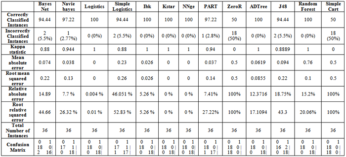
- Table 1 present the Classification of colon cancer dataset using weka 3.6, in which Logistics, Ibk, Kstar, NNge, ADTree, Random Forest Algorithms show 100 % correctly classified instances, followed by Navie Bayes and PART with 97.22 %, Simple Cart and ZeroR has shown the least with 50 % of correctly classified instances. Kappa Statistic for Logistics, Ibk, Kstar, NNge, ADTree, Random Forest has shown Maximum. Mean absolute error is low for Logistics,Kstar, NNge. Root mean squared error is low for Logistics, Kstar and NNge.
|
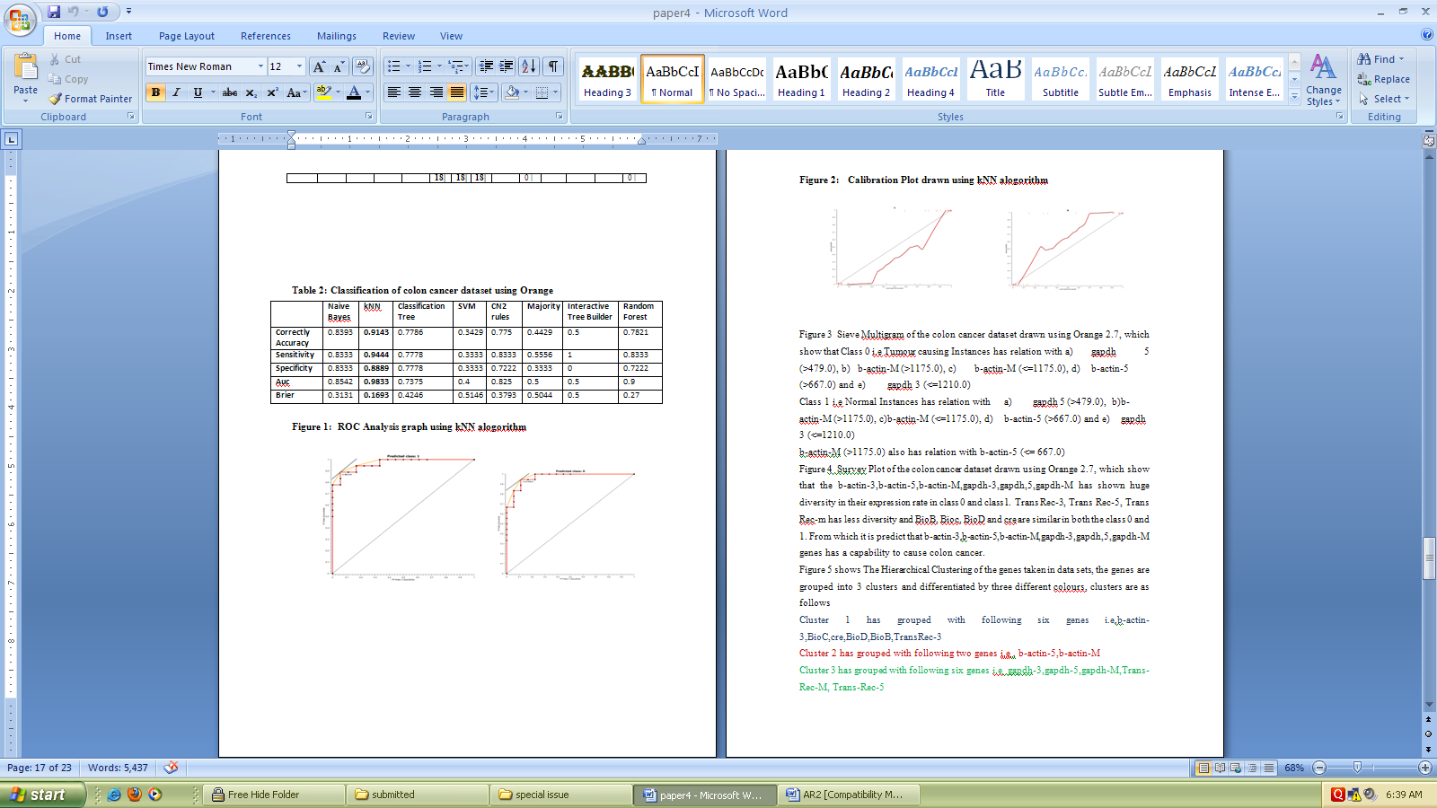 | Figure 1. ROC Analysis graph using kNN alogorithm |
 | Figure 2. Calibration Plot drawn using kNN alogorithm |
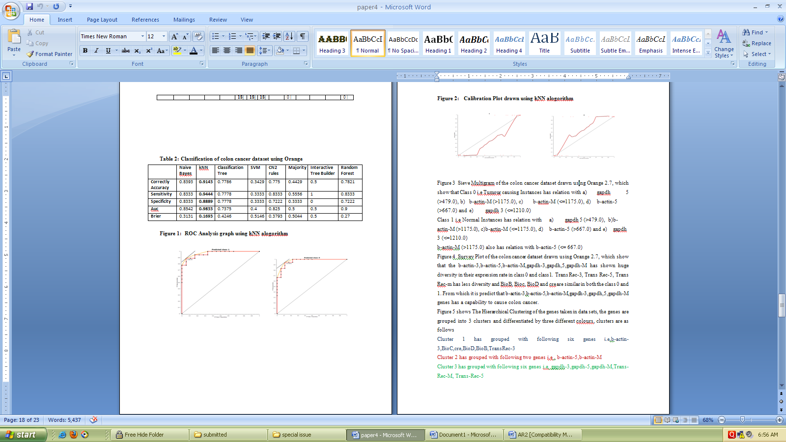
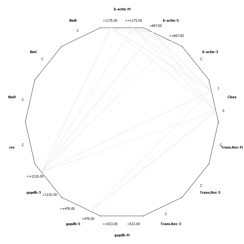 | Figure 3. Sieve Multigram |
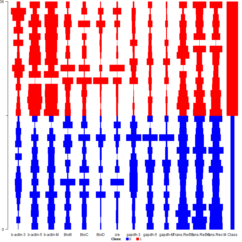 | Figure 4. Survey Plot |
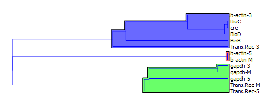 | Figure 5. Hierarchical Clustering |
4. Discussion
- Colorectal cancer (cancer of the colon or rectum) is the third most commonly diagnosed cancer in males and the second in females, with over 1.2 million new cancer cases and 608,700 deaths estimated to have occurred in 2008 The highest incidence rates are found in Australia and New Zealand, Europe, and North America, where as the lowest rates are found in Africa and South-Central Asia[26, 29, 30]. The exact cause of colorectal cancer is unknown, in fact it is thought that there is not one single cause. It is more likely that a number of factors, some known and many unknown, may work together to trigger the development of colorectal cancer. Previous studies have identified risk factors which may increase a person’s risk of developing colorectal cancer[31].Supervised learning involves:1. Classification: Classification is learning a function that maps (classifies) a data item into one of several predefined classes.2. Estimation: Given some input data, coming up with a value for some unknown continuous variable.3. Prediction: Same as classification & estimation except that the records are classified according to some future behaviour or estimated future value.Un-Supervised learning involves :1. Association rules: Determining which things go together, also called dependency modeling.2. Clustering: Segmenting a population into a number of subgroups or clusters.3. Description & visualization: Representing the data using visualization techniques.4. The primary goals of data mining, in practice, are prediction and description. These main tasks are well suited for data mining, all of which involves mining a meaningful new patterns from the existing data, Learning from data falls into two categories: directed (“supervised”) and undirected (“unsupervised”) learning.DNA microarrays dataset contains information about gene expression, differences in tissues and cell samples. The knowledge about genetic variation that appears in the samples allows for disease diagnosis or building new hypothesis about gene to gene relations in organisms. In here data mining techniques are also used for the identification of the most informative genes. One of the most challenging problems with gene expression mining is dimensionality reduction and specific variation in the data. The methods frequently used for microarray analysis are Classification algorithms, SVM, hierarchical clustering, neural networks and statistical measures are used for its optimizations. The Notterman Carcinoma dataset is subjected for statistical analysis where the clustering analysis has shown that b-actin-5,b-actin-M are closely related b-actin-3, BioC, cre, BioD, BioB, Trans-Rec-3 are closely related and belongs to class 1(predict positive) gapdh-3, gapdh-5, gapdh-M, Trans-Rec-M, Trans-Rec-5 belongs to class 0 (predict negative).
5. Conclusions
- Data mining approaches seem ideally suited for bioinformatics, since bioinformatics is data-rich but lacks a comprehensive theory of life’s organization at the molecular level. Data mining is used in various medical applications, The present research work on Colon Cancer dataset showed that Logistics, Ibk, Kstar, NNge, ADTree, Random Forest Algorithms are the best suited algorithms for the classification analysis and Hierarchical Clustering method is used for the clustering analysis.
ACKNOWLEDGEMENTS
- Authors would like to thank management and staff of GITAM University and Dr.LB PG College, India for their kind support in bringing out the above literature and providing lab facilities.
References
| [1] | Mohammed J. Zaki, Shinichi Morishita, Isidore Rigoutsos, “Report on BIOKDD04: Workshop on Data Mining in Bioinformatics”, in SIGKDD Explorations, vol. 6, no. 2, pp. 153-154, 2004. |
| [2] | J. Li, L. Wong, Q. Yang, “Data Mining in Bioinformatics”, IEEE Intelligent System, IEEE Computer Society. Indian Journal of Computer Science and Engineering, vol 1 no 2, pp. 114-118, 2005. |
| [3] | R. P. Kumar, M. Rao, D. Kaladhar, “Data Categorization and Noise Analysis in Mobile Communication Using Machine Learning Algorithms”, Wireless Sensor Network, vol. 4, no.4, pp. 113-116, 2012. |
| [4] | Mark H. E. Frank, Geoffrey Holmes, Bernhard Pfahringer, Peter Reutemann, Ian H. Witten, “The WEKA data mining software: an update“, SIGKDD Explorations, vol. 11, no.1, pp.10-18, 2009. |
| [5] | D. J. Hand, “Statistics and data mining: intersecting disciplines“, SIGKDD Explorations, vol. 1, no. 1, pp. 16-19, 1999. |
| [6] | C Apte, E Grossman, E Pednault, B Rosen, F Tipu, B White, "Insurance risk modeling using data mining technology", Proceedings of PADD99: The Practical Application of Knowledge Discovery and Data Mining, pp.39-47, 1999. |
| [7] | Liu, Bing, Chee Wee Chin, Hwee Tou Ng. "Mining topic-specific concepts and definitions on the web." Proceedings of the 12th international conference on World Wide Web. ACM, pp.251-260, 2003. |
| [8] | M.K. Jakubowski, Q. Guo, M. Kelly, “Tradeoffs between lidar pulse density and forest measurement accuracy”, Remote Sensing of Environment, vol. 130, pp. 245-253, 2013. |
| [9] | E. Frank, M. Hall, L. Trigg, G. Holmes, I. H. Witten, “Data mining in bioinformatics using Weka”, Bioinformatics, vol. 20, no. 15, pp. 2479-2481, 2004. |
| [10] | M. Hall, E. Frank, G. Holmes, B. Pfahringer, P. Reutemann, I. H. Witten, “The WEKA data mining software: an update”, ACM SIGKDD Explorations Newsletter, vol. 11, no. 1, pp. 10-18, 2009. |
| [11] | Tomaž Curk, Janez Demšar, Qikai Xu, Gregor Leban, Uroš Petrovič, Ivan Bratko, Gad Shaulsky, Blaž Zupan, “Microarray data mining with visual programming”, Bioinformatics, vol. 21, no. 3, pp. 396-398, 2005. |
| [12] | R. W. Burt, J. S. Barthel, K. B. Dunn, D. S. David, E. Drelichman, J. M. Ford, et al, “Colorectal cancer screening”, Journal of the National Comprehensive Cancer Network, vol. 8, no. 1, pp. 8-61, 2010. |
| [13] | David Cunningham, Wendy Atkin, Heinz-Josef Lenz, Henry T Lynch, Bruce Minsky, Bernard Nordlinger, Naureen Starling, “Colorectal cancer”, The Lancet, vol. 375, no. 9719, pp. 1030-1047, 2010. |
| [14] | R. A. Smith, V. Cokkinides, D. Brooks, D. Saslow, O. W. Brawley, “Cancer screening in the United States, 2010: a review of current American Cancer Society guidelines and issues in cancer screening”, CA: a cancer journal for clinicians, vol. 60, no.2, pp. 99-119, 2010. |
| [15] | K. Mehmed, "Data Mining: Concepts, Models, Methods And Algorithms." IEEE Computer Society, IEEE Press, 2003. |
| [16] | W. J. Frawley, G. Piatetsky-Shapiro, C. J. Matheus, “Knowledge discovery in databases: An overview”, AI magazine, vol. 13, no. 3, pp. 57, 1992. |
| [17] | H. Lieberman, D. Maulsby, “Instructible agents: Software that just keeps getting better”, IBM Systems Journal, vo. 35, no. 3.4, pp. 539-556, 1996. |
| [18] | R. Rada, “Expert systems and evolutionary computing for financial investing: A review”, Expert systems with applications, vol. 34, no. 4, pp. 2232-2240, 2008. |
| [19] | Cho Sung-Bae, Hong-Hee Won, "Machine learning in DNA microarray analysis for cancer classification", In Proceedings of the First Asia-Pacific bioinformatics conference on Bioinformatics, vol. 19, pp. 189-198. 2003. |
| [20] | Goebel Michael and Le Gruenwald. "A survey of data mining and knowledge discovery software tools", ACM SIGKDD Explorations Newsletter vol. 1, no. 1, pp. 20-33, 1999. |
| [21] | A. Chaiboonchoe, S. Samarasinghe, D. Kulasiri, “Machine Learning for Childhood Acute Lymphoblastic Leukaemia Gene Expression Data Analysis: A Review”, Current Bioinformatics, vol. 5, no.2, pp. 118-133, 2010. |
| [22] | DSVGK Kaladhar, B. Chandana, “Data Mining, inference and prediction of Cancer datasets using learning algorithms”, International Journal of Science and Advanced Technology, vol. 1, no.3, pp. 68-77, 2011 |
| [23] | H. John George, Pat Langley, "Estimating continuous distributions in Bayesian classifiers." In Proceedings of the eleventh conference on uncertainty in artificial intelligence, pp. 338-345. Morgan Kaufmann Publishers Inc., 1995. |
| [24] | Chang Chih-Chung, Chih-Jen Lin, "LIBSVM: a library for support vector machines", ACM Transactions on Intelligent Systems and Technology (TIST), vol. 2, no. 3, pp. 27, 2011. |
| [25] | Jemal Ahmedin, Freddie Bray, Melissa M. Center, Jacques Ferlay, Elizabeth Ward, David Forman, "Global cancer statistics", CA: a cancer journal for clinicians, vol. 61, no. 2, pp. 69-90, 2011. |
| [26] | A. Notterman Daniel, Uri Alon, Alexander J. Sierk, Arnold J. Levine, "Transcriptional gene expression profiles of colorectal adenoma, adenocarcinoma, and normal tissue examined by oligonucleotide arrays", Cancer Research, vol. 61, no. 7, 3124-3130, 2001. |
| [27] | Vuk Miha, Tomaz Curk. "ROC curve, lift chart and calibration plot." Metodoloski zvezki, vol. 3, no. 1, pp. 89-108, 2006. |
| [28] | Yu, Yunxian, Yifeng Pan, Mingjuan Jin, Mingwu Zhang, Shanchun Zhang, Qilong Li, Xia Jiang et al. "Association of genetic variants in tachykinins pathway genes with colorectal cancer risk." International Journal of Colorectal Disease (2012): 1-8. |
| [29] | Desai Monica Dandona, Bikramajit Singh Saroya, Albert Craig Lockhart, "Investigational therapies targeting the ErbB (EGFR, HER2, HER3, HER4) family in GI cancers", Expert opinion on investigational drugs, vol. 0, pp. 1-16, 2013. |
| [30] | Penninx, Brenda WJH, Jack M. Guralnik, Richard J. Havlik, Marco Pahor, Luigi Ferrucci, James R. Cerhan, Robert B. Wallace, "Chronically depressed mood and cancer risk in older persons", Journal of the National Cancer Institute, vol. 90, no. 24, pp. 1888-1893, 1998. |