Tzvetalin S. Vassilev , Laura Huntington
Department of Computer Science and Mathematics, Nipissing University, North Bay, P1B 8L7, Canada
Correspondence to: Tzvetalin S. Vassilev , Department of Computer Science and Mathematics, Nipissing University, North Bay, P1B 8L7, Canada.
| Email: |  |
Copyright © 2012 Scientific & Academic Publishing. All Rights Reserved.
Abstract
This paper explores maximum as well as optimal matchings with a strong focus on algorithmic approaches to determining these matchings. It begins with some basic terminology and notions about matchings including Berge’s Theorem, Hall’s Theorem and the König-Egerváry Theorem among others. Then an algorithm used for determining maximum matchings in bipartite graphs is discussed and examples of its execution are explored. This discussion is followed by an exploration of weighted graphs and optimal matchings including a statement and discussion of the Hungarian Algorithm. The Marriage Algorithm is also discussed as are stable marriages and examples of the execution of the Marriage Algorithm are provided.
Keywords:
Graph Theory, Matchings, Greedy Algorithms, Stable Marriage
Cite this paper:
Tzvetalin S. Vassilev , Laura Huntington , "Algorithms for Matchings in Graphs", Algorithms Research , Vol. 1 No. 4, 2012, pp. 20-30. doi: 10.5923/j.algorithms.20120104.02.
1. Introduction
There are many different interesting applications of matchings to all aspects of life – from how to fill positions at a place of business with the best possible combination of applicants to how to ensure that a ‘marriage’ is stable! Of course, this is assuming that a person’s suitability for a specific role, whether it is as a new employee or a spouse to a certain person, can be easily determined and quantified which clearly is not always the case. However, we will conveniently consider an optimal and easily quantifiable world throughout this paper in which one will never hire an employee who is not suitable for a position and the divorce rate is considerably lower!
2. Basic Terminology and Properties of Matchings
2.1. Matchings Terminology
A set of pairwise independent edges is called a matching. Edges are called independent if they are not adjacent. In the study of matchings, the notion of a maximal matching becomes interesting. A matching of maximum cardinality is called a maximum matching and a matching that pairs all the vertices in a graph is called a perfect matching (see Figure 1). Thus, it makes sense to seek not only a matching but the largest possible matching by some measurable quantity[1]. A common practical application of such a problem is one considering jobs and applicants. Suppose that there are m positions to be filled at a particular company for which the company has n applicants. If we assign each position and each applicant a vertex we can attempt to find a matching in this bipartite graph. A bipartite graph is a graph whose vertices can be separated into two sets X and Y in such a way that every edge in the graph has one endpoint in each set[2]. In this case, the two sets would be the set P such that |P|=m and the set A such that |A|=n since there are m positions and n applicants. 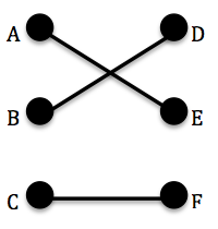 | Figure 1. Matching in a bipartite graph |
Also, note that the neighbourhood of a vertex v in a graph G is an induced subgraph of G, formed by all vertices adjacent to v. Denoted N(v) such that the number of vertices adjacent to v is |N(v)|[3].
2.2. Types of Edges, Vertices and Paths in a Matching
An edge is defined to be weak with respect to a matching M if it is not in the matching[1]. For example, let G be the graph in Figure 1. Let M be the set {AE, CF} where AE denotes an edge from vertex A to vertex E. Then the edge BD is weak with respect to the matching M since BD is not included in the set M of pairwise independent edges. A vertex is weak with respect to M if it is incident to only weak edges. Again, given the above-described matching M in Figure 1, the vertices B and D are weak with respect to the matching M since B and D are incident only to BD which, as already established, is a weak edge with respect to M.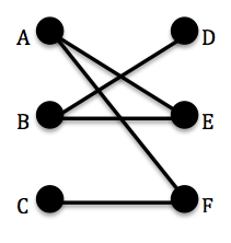 | Figure 2. Alternating paths and matchings |
An M-alternating path in G is a path whose edges are alternately in a matching M and not in M[1]. Consider the following graph G in Figure 2 and the matching M={AE, BD, CF}. An M-alternating path in G is given by: CF, FA, AE, EB, BD. An M-augmenting path is an M-alternating path whose end vertices are both weak with respect to M[1]. Note that there is no possible M-augmenting path in the graph G in Figure 2 since G has no vertices that are weak with respect to M. If we redefined M={AE} then an M-augmenting path in G would be given by: FA, AE, EB since in this case F and B would be weak vertices with respect to this particular matching M.
2.3. Some Properties of Matchings
Lemma 1 Let M1 and M2 be two matchings in a graph G. Then each component of the spanning subgraph H with edge set  is one of the following types:1. An isolated vertex.2. An even cycle with edges alternately in M1 and M2.3. A path whose edges are alternately in M1 and M2 and such that each end vertex of the path is weak with respect to exactly one of M1 and M2[1] .Proof: Let M1 and M2 be two matchings in a graph G. Let H be a spanning subgraph of G with edge set
 . H is the union of the edges which are in M1 and not in M2 and the edges which are in M2 and not in M1.Now, in the subgraph H of G,
  . Otherwise, a vertex in H would have to be adjacent to more than 1 edge from at least one of the matchings. Thus, the possible components of H are isolated vertices, paths and cycles.Consider a component H1 of H that is not an isolated vertex. This component is either a path or a cycle.Obviously an edge in H1, must either be from M1 or M2, it cannot be from both by the definition of E(H). Also, consider a vertex v in H1. Since
 ,
,  which means that there are at most two edges incident to v. These edges cannot be both from the same matching, M1 or M2, otherwise the definition of matching would not be satisfied. Thus, the edges in this component H1 of H are alternating between the two matchings. Therefore, if H1 is a cycle, then it must be an even cycle with edges alternating between M1 and M2. (Otherwise, the edges would not alternate and at least one vertex would have more than one edge from one of the matchings).By the same reasoning, if H1 is a path, the edges in the path would have to be alternating between the two matchings. It remains to be shown that each end vertex is weak with respect to exactly one of the matchings. In other words, we must show that each end vertex has only one edge incident to it.Suppose not. Suppose v is a vertex in H1 was also adjacent to an edge e from the other matching. Then we could extend the path and v would not be the end vertex.
2.4. Matching Theorems
Theorem 1 (Berge’s Theorem) A matching M in a graph G is a maximum matching if, and only if, there exists no M-augmenting path in G.Proof: Let M be a matching in G and suppose that G contains an M-augmenting path  .Note that k must be odd because P is an M-augmenting path which means that its edges alternate between those in the matching M and those not in the matching M and that each of its end vertices are weak with respect to M. Consider the matching M and the M-augmenting path given by P. Let us remove all the edges from M which are in P. Then let us add the edges which were weak with respect to M in P to construct a new matching: M1 = {v1,v2,…,vk-2,vk-1} U { v0,v1,…,vk-1,vk}.Now since v0 and vk were the end vertices of P, they were weak with respect to M. This means that {v0,v1,…,vk-1,vk} with what remains of M, which we defined as M1 is a set of pairwise independent edges in G and thus M1 is a matching in G. Note that k -1 is always even under these assumptions.In order to find M1 we removed (k – 1)/2 edges from M and then added (k +1)/2 edges. Note that[(k +1)/2]–[(k – 1)/2] = 1.Thus, M1 is a matching in G which contains one more edge than M and so M is not a maximum matching in G.Conversely, suppose that M is not a maximum matching and there does not exist an M-augmenting path. Using the same M1, let M1 be a maximum matching in G. Consider the spanning subgraph H as defined in Lemma 1 but between M1 and M. As it was proven, H must either be an isolated vertex, an even cycle with edges alternately in M1 and M, or a path whose edges are alternately in M1 and M such that each end vertex of the path is weak with respect to exactly one of M1 and M. Consider a component of H which is an alternating path. Its end vertices must be weak with respect to exactly one of M1 and M. But some alternating path in H must contain more edges of M1 than M, since M1 contains more edges than M. Thus, this path is an M-augmenting path but we assumed that there was no such path possible.Given a matching M, a set S is matched under M if every vertex of S is incident to an edge in M[1].Theorem 2 (Hall’s Theorem) Let
  be a bipartite graph. Then X can be matched to a subset of Y if, and only if, |N(S)| is greater than or equal to |S| for all subsets S of X[1].Proof: Suppose that X can be matched to a subset Y. Consider a vertex vi in S. For each vertex vi in S, vi is adjacent to at least one vertex in Y. Thus, each vertex vi in S contributes at least one vertex to N(S). Now, the size of the subset S, denoted |S|, is the number of vertices vi in S. And since each of these vertices contribute at least one vertex to the neighbourhood of S, it follows that |N(S)| greater than or equal to |S| for all subsets S of X.Conversely, suppose X cannot be matched to a subset Y. We need to show that |N(S)| being greater than or equal to |S| for all subsets S of X does not hold. Let M be a maximum matching in a graph G. Now, obviously all the vertices of X cannot be incident to edges in M since X cannot be matched to Y. So there is at least one vertex in X that is weak with respect to M. Let u be a vertex in X that is weak with respect to M. Let A be the set of all vertices of the graph G which are connected to u by an M-alternating path. Now, since M is a maximum matching by our assumption, it follows that there is no M-augmenting path in G by Berge’s Theorem (Theorem 1). Which means that there can be no vertex in A, other than u, that is weak with respect to the matching M otherwise there would be an M-augmenting path in G and thus M would not be a maximum matching.Let S = A ∩ X and T = A ∩ Y. The vertices of S – {u} are matched with vertices of T, since u is the only weak vertex in A with respect to the maximum matching M. Therefore |T| = |S| - 1 since all the vertices in S other than u must be in T. In fact
  since every vertex in N(S) is connected to u by an alternating path. But then |N(S)| = |S| - 1 which is less than |S|.Corollary 1 (to Hall’s Theorem) If G is a k-regular bipartite graph with
 , then G has a perfect matching.Proof: Let G = (X U Y, E) be a k-regular bipartite graph with
 .Then the number of edges in G will equal k multiplied by the number of vertices in X and k multiplied by the number of vertices in Y,
 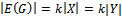 . Thus, since
 , X and Y have the same number of vertices.If S is a subset of X, since we know that |N(S)| is greater than or equal to |S|, it follows that the set of all edges incident to vertices in S, denoted Es, is a subset of all the edges incident to the vertices in N(S), denoted EN(S). In other words,
  .Now, G is k-regular so k|N(s)| =|EN(S)| , and from above, k|N(s)| =|EN(S)| which is greater than or equal to | Es| = k|S|. It follows that |N(S)| is greater than or equal to |S| and thus, by Hall’s Theorem, X can be matched to subset of Y. But we have already established that there are the same number of vertices in the sets X and Y so G must contain a perfect matching.
2.5. The SDR and the Marriage Theorems
Hall’s Theorem can also be stated in set theoretic terms. We shall state it in these terms as it will be very useful in this form in later discussions. However, before this statement can be made, we need to establish a few more terms and their definitions.Given sets S1, . . . , Sk let  be any element such that we define xi is a representative for the set Si which contains it. A collection of distinct representatives for this set is called a system of distinct representatives (aka.‘SDR’) or a transversal of sets. Theorem 3 (The SDR Theorem) A collection S1, S2, . . . , Sk, k ≥ 1 of finite nonempty sets has a system of distinct representatives if, and only if, the union of any t of these sets contains at least t elements for each t, (1 ≤ t ≤ k)[1].Proof: If the union of any t of these sets contained less than t elements then there would be fewer elements to be chosen as the representatives than there are sets to be represented.Theorem 4 (The Marriage Theorem) Given a set of n men and a set of n women, let each man make a list of the women he is willing to marry. Then each man can be married to a woman on his list if, and only if, for every value of k ( 1 ≤ k ≤ n ), the union of any k of the lists contain at least k names[1].A set C of vertices is said to cover the edges of a graph G (or be an edge cover), if every edge in G is incident to a vertex in C[2].There are some very useful results relating edge covers and matchings. One such result is the König-Egerváry theorem.Theorem 5 (König-Egerváry Theorem) If
  is a bipartite graph, then the maximum number of edges in a matching in G equals the minimum number of vertices in a cover for E(G), that is, α(G) = β(G).Proof: Let
  be a bipartite graph. Suppose that the maximum number of edges in a matching in G is m, denoted α (G) = m and suppose that the minimum number of vertices in a cover for E(G) is c, denoted β(G) = c. We want to show that m = c.Let M be a maximum matching in G. Let W be the set of all vertices in X which are weak with respect to the matching M. Thus the size of the matching is the size of X minus that size of W. Let the set S contain all the vertices of G which are connected to some vertex in W by an alternating path. Let Sx =S ∩ X and let Sy =S ∩ Y.Since S contains the vertices in G with are connected to the vertices of W by an alternating path and since W is the set of all vertices of X which are weak with respect to the matching, this implies that no vertex in Sx - W is weak. This in turn implies that Sx - W is matched under M to Sy and that N(Sx) = Sy. Thus |Sx| - |Sy| = |W|.Then we claim that C = (X – Sx) U Sy is a cover for E(G). Suppose not, that is suppose C was not a cover for E(G), then there would have to be an edge vw in G where v is an vertex in Sx and w is a vertex that is not in Sy = N(Sx) which is not possible. (There would be an edge between a vertex in one set and a vertex which was not in the neighbourhood of the set).Therefore we would have the following:|C| = |X| - |Sx| + |Sy| = |X| - |W| = |M|.Thus, c = m.
3. An Algorithm for Determining Maximum Matchings in Bipartite Graphs
Algorithm 1 A Maximum Matching in a Bipartite Graph[1].Input: Let  be a bipartite graph and suppose that X = { x1, . . . , xm } and Y = { y1, . . . , yn }. Further, let M be any matching in G (including the empty matching). Output: A matching larger than M or the information that the present matching is maximum.
Method: We now execute the following labeling steps until no step can be applied.1. Label with an * all vertices of X that are weak with respect to M. Now, alternately apply steps 2 and 3 until no further labeling is possible. 2. Select a newly labelled vertex in X, say xi, and label with xi all unlabeled vertices of Y that are joined to xi by an edge weak with respect to M. Repeat this step on all vertices of X that were labeled in the previous step. 3. Select a newly labelled vertex of Y, say yj, and label with yj all unlabeled vertices of X which are joined to yj by an edge in M. Repeat this process on all vertices of Y labeled in the previous step.
be a bipartite graph and suppose that X = { x1, . . . , xm } and Y = { y1, . . . , yn }. Further, let M be any matching in G (including the empty matching). Output: A matching larger than M or the information that the present matching is maximum.
Method: We now execute the following labeling steps until no step can be applied.1. Label with an * all vertices of X that are weak with respect to M. Now, alternately apply steps 2 and 3 until no further labeling is possible. 2. Select a newly labelled vertex in X, say xi, and label with xi all unlabeled vertices of Y that are joined to xi by an edge weak with respect to M. Repeat this step on all vertices of X that were labeled in the previous step. 3. Select a newly labelled vertex of Y, say yj, and label with yj all unlabeled vertices of X which are joined to yj by an edge in M. Repeat this process on all vertices of Y labeled in the previous step. 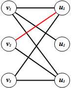 | Figure 3. The initial matching |
Notice that the labelings will continue to alternate until one of two possibilities occurs:E1 : A weak vertex in Y has been labeled.
E2 : It is not possible to label any more vertices and E1 has not occurred.Let us now apply this algorithm to the following bipartite graph G to find a maximum matching in G.Input:  where V = {v1, v2, v3} and U = {u1, u2, u3}. Let M = {v2u1} be matching in G.1. Label with an * all vertices of V that are weak with respect to M. ● These are all the vertices in V which are not in M; that is, v1 and v3.
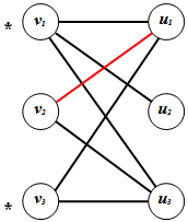 | Figure 4. The labeling after Step 1 |
2. Select a newly labelled vertex in V, say vi, and label with vi all unlabeled vertices of U that are joined to vi by an edge weak with respect to M. Repeat this step on all vertices of V that were labelled in the previous step.● Let us select v1 first. The unlabelled vertices of U which are adjacent to v1 are u1, u2 and u3. We label these three vertices with v1.● Now we consider v3. Since v3 is only adjacent to vertices in U which are already labelled, no further labelling can be done at this step3. Select a newly labelled vertex of U, say uj, and label with uj all unlabeled vertices of V which are joined to uj by an edge in M. Repeat this process on all vertices of U labelled in the previous step. ● The only vertex in V which has not been labelled yet is v2 so let us choose a vertex in U that was labelled in the previous step that is adjacent to v2.● Choose u1. We must now label v2 with u1.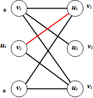 | Figure 5. The labelling after Step 3 |
Note: Here we reach the end of this execution of the algorithm. Since weak vertices with respect to M in U were labelled, the ending E1 has occurred. Also, the path P: v1u2 is augmenting (starts and ends on vertices which are weak with respect to M). So our new matching is M’={v2u1, v1u2}.Now we run the algorithm again, this time starting with the matching M’={v2u1, v1u2}.1. v3 is the only vertex in V which is weak with respect to M’.● Now we label all the vertices in U which are adjacent to v3 with v3. These would be u1 and u3.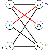 | Figure 6. The new matching M’ and the labelling after Step 1 |
2. Now we choose u1 and label v1 and v2 with u1. ● Note that if we now choose u3, it is only adjacent to vertices in V that are already labelled so we need not consider it.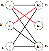 | Figure 7. The labelling after Step 2 |
3. Consider v1. It is adjacent to u2 in U which as of the previous step was unlabelled so we label u2 with v1.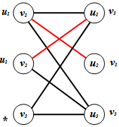 | Figure 8. The labelling after Step 3 |
This second pass of the algorithm halts here because all the vertices in G have been labelled. Note that the ending here is again E1 since it resulted in the labelling of u3 which is a weak vertex in U with respect to M’.Now we have the path P’ = {v3u3} which is augmenting and we form the new matching M’’ = {v2u1, v1u2, v3u3}. When we run the algorithm once more with the matching M’’ = {v2u1, v1u2, v3u3}, (as depicted with the red edges), we immediately find that there are no vertices in V that are weak with respect to M’’ and thus the algorithm halts with ending E2.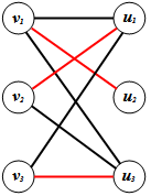 | Figure 9. The matching M” |
Now we will prove the following theorem, which states that since the algorithm terminated with ending E2, M’’ is a maximum matching in G.
3.1. Proof that Algorithm 1 Outputs a Maximum Matching if it Terminates with Ending E2
Theorem 6 Let G be a bipartite graph with a matching M. Suppose that the above algorithm has halted with ending E2 occurring. Let Ux be the unlabeled vertices in X and Ly be the labelled vertices in Y. Then C = Ux U Ly covers the edges of G, |C| = |M|, and M is a maximum matching in G.Proof: Suppose not; that is suppose C = Ux U Ly does not cover the edges of G. Then there exists and edge from a labelled vertex of X to an unlabelled vertex in Y. Call this edge e = xy where x is an element of Lx and y is an element of Uy. If e is not in M, then since x is labelled, it follows from step 2 of the algorithm that y is labelled. But y is in Uy from our definition of y. This means that e must be in M and thus, from step 3 of the algorithm, x must be labeled with y. This also means that y must have been labeled in a previous step. But again y is in Uy from our definition of y. Therefore, there cannot be edges from a labeled vertex in X to an unlabeled vertex in Y so C must cover all the edges of G.Let us consider what this theorem and its proof mean in terms of our example. If we let Uv be the unlabelled vertices of V and Lu be the labelled vertices of U. According to Theorem 4, C = Uv U Lu should cover the edges of G. In our example, none of the vertices in V are weak with respect to M’’ so all the vertices in V are unlabelled and thus will be included in C; on the other hand, since the algorithm halted on the first step, none of the vertices of U were labelled and thus none of the vertices in U are included in C. Therefore, C = {v1, v2, v3} and since there are no isolated vertices in G, and G is bipartite, C does cover all the edges of G. Now |C|=3 and we found the matching: M’’ = {v2u1, v1u2, v3u3}, where |M’’| = 3 . Thus, |C| = |M’’|. And so M’’ is a maximum matching in G.
4. Assigning Weights and Determining Optimal Solutions
4.1. Introduction
It now becomes interesting to take the notion of a maximum matching and apply it to a more complicated but also more useful notion of an optimal matching in a graph with weighted edges. For example, given the jobs and applicants problem presented in section 2.1, forming a maximum matching in this situation would only ensure that the maximum possible number of jobs were filled (or the maximum number of applicants were hired); this matching would not even begin to consider the optimal solution in any terms except quantity. A common consideration in the hiring process is the suitability of an applicant for a job. If each applicant’s suitability (or unsuitability) for each job was calculated in some way, then one could attempt to find a solution which would ensure the optimal assigning of applicants to jobs in terms of suitability (or unsuitability). To explore these optimal matchings, we discuss weighted edges. A weighted edge in a graph is an edge that has number or weight assigned to it. A weighted graph then, is a graph in which each edge has a number associated with it[1]. Then, to find this optimal matching, one must determine a matching with a collection of edges for which the sum of the weights of these edges is either minimal or maximal depending on the significance behind the weights on each edge and the specific characteristics of the solution being optimized. In the jobs and applicants example, suppose that there are m positions to be filled at a particular company for which the company has n applicants. As with the general matching, we assign each position and each applicant a vertex and we can attempt to find a matching in this bipartite graph. However, we now take into account each applicant’s unsuitability for each job. Let a weight of 0 indicate that the applicant is perfectly suited to a job and let an increase in the weight of each edge indicate an increase in unsuitability of an applicant to a job. In such a way, we can now consider the optimal matching which would result in the best possible allocation of the jobs to the most suitable applicants overall. Note that this optimization does not necessarily result in each applicant being offered the job for which they are best suited for the simple reason that there may be more than one applicant whose is equally highly suited to the job. To optimize this matching, we must then determine the matching for which the sum of the weights of the edges in the matching is minimized, meaning that the unsuitability of the applicants to the jobs to which they are assigned in this matching is minimized.Let us define the weight of a matching M to be the sum of the weights of each of the edges e in M, where w(e) is the weight assigned to the edge e. In this way, an optimal solution is a perfect matching in which W(M) is minimal[1].Note: The bipartite graph in these examples will be complete, since we must consider the unsuitability of every applicant to every job. If an applicant is completely unsuitable for a job or did not apply for a job, we have the option of weighting the edge between that job and that applicant high enough that it would never be considered in the optimization. Sometimes these edges are given infinite weight, denoted by ∞.Consider the following graph H: 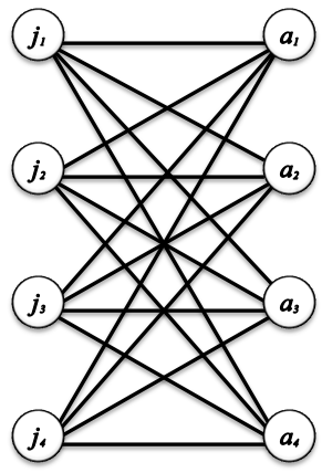 | Figure 10. Jobs and applicants, the graph H |
As noted above, H is a complete bipartite graph. In this case there are 4 applicant and 4 jobs to be filled.Now, to write on the graph the weight of each edge would be difficult to do and to read and thus we will use the following table:| Table 1. The weights in the graph H |
| | U | a1 | a2 | a3 | a4 | | j1 | 5 | 7 | 2 | 0 | | j2 | 1 | 9 | 10 | 4 | | j3 | 7 | 8 | 1 | 11 | | j4 | 0 | 3 | 4 | 5 |
|
|
The next logical step in our search for the optimal solution would be to try to simplify the weights of the edges in this table. Note what happens if we subtract the same amount from every entry in one row or column. For instance, let us subtract 1 from each of the entries in row j2. The new table becomes:| Table 2. The simplified weights after subtraction of 1 from row j2 |
| | U | a1 | a2 | a3 | a4 | | j1 | 5 | 7 | 2 | 0 | | j2 | 0 | 8 | 9 | 3 | | j3 | 7 | 8 | 1 | 11 | | j4 | 0 | 3 | 4 | 5 |
|
|
Essentially, we have not actually changed the relative unsuitability of the applicants for this job since we decreased each weight by the same amount.When we consider that only one entry from each column will be selected when calculating W(M), we can conclude this change will have the same effect on any M that is chosen and thus we can simplify the table in such a way.So for each of the remaining rows, select the least entry in the row and subtract it from all the entries in that row. (Note that we use the least entry in each row in order to eliminate the occurrence of negative weights). For instance, in row j3 the smallest entry is 1 so we subtract 1 from 7, 8, 1, and 11 to form the new table:| Table 3. Simplification in all rows |
| | U | a1 | a2 | a3 | a4 | | j1 | 5 | 7 | 2 | 0 | | j2 | 0 | 8 | 9 | 3 | | j3 | 6 | 7 | 0 | 10 | | j4 | 0 | 3 | 4 | 5 |
|
|
Note that in rows j1 and j4 the smallest entry is already 0 so these rows remain unchanged. (Subtracting 0 from a row will result in no change to that row).Now let us repeat this process with the columns of the table; that is, in each column, subtract the least entry from all of the entries. The following table is formed:| Table 4. After the column simplification |
| | U | a1 | a2 | a3 | a4 | | j1 | 5 | 4 | 2 | 0 | | j2 | 0 | 5 | 9 | 3 | | j3 | 6 | 4 | 0 | 10 | | j4 | 0 | 0 | 4 | 5 |
|
|
Now we must select numbers from the table, no two from the same row or column, with as small a sum as possible[1]. We eliminated the possibility of negative weights so the minimum sum we could have is 0.If we select the following entries marked with an asterisk (*), we will have a sum of zero and no entry selected will be in the same row or column as any other entry selected.| Table 5. Selection corresponding to an optimal matching |
| | U | a1 | a2 | a3 | a4 | | j1 | 5 | 4 | 2 | 0* | | j2 | 0* | 5 | 9 | 3 | | j3 | 6 | 4 | 0* | 10 | | j4 | 0 | 0* | 4 | 5 |
|
|
Thus, we establish the following optimal solution M = {j2a1, j4a2, j3a3, j1a4}.
4.2. Exceptions/Difficulties and the Hungarian Algorithm
Unfortunately, we will not always be lucky enough to obtain entries for which there are n “independent 0’s”. Consider the following table of edge weights:| Table 6. Alternative weight assignment for the graph H |
| | U | a1 | a2 | a3 | a4 | | j1 | 2 | 7 | 8 | 13 | | j2 | 3 | 5 | 14 | 10 | | j3 | 11 | 9 | 7 | 6 | | j4 | 5 | 3 | 9 | 11 |
|
|
After subtracting the least weight from each row of the table we have the following table:| Table 7. After the row simplification |
| | U | a1 | a2 | a3 | a4 | | j1 | 0 | 5 | 6 | 11 | | j2 | 0 | 2 | 11 | 7 | | j3 | 5 | 4 | 1 | 0 | | j4 | 2 | 0 | 6 | 8 |
|
|
And then repeating this with the columns of the table yields:| Table 8. After the column simplification |
| | U | a1 | a2 | a3 | a4 | | j1 | 0 | 5 | 5 | 11 | | j2 | 0 | 2 | 10 | 7 | | j3 | 5 | 4 | 0 | 0 | | j4 | 2 | 0 | 5 | 8 |
|
|
Note that in this table there is no set of 4 independent zeroes and, unlike the previous example, at this step we cannot immediately determine an optimal matching.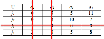 | Figure 11. Crossing out the rows with zeroes in Table 8 |
Gould gives the following ‘adjustment procedure’ which can be used to determine a set of independent zeroes[1].First we must cross out with a line all the rows and columns in the table containing zeroes.Then the following algorithm must be run (this algorithm is often known as the Hungarian Algorithm in honor of König and Egerváry):Algorithm 2 (The Hungarian Algorithm)1. Let m be the smallest number that is not included in any of our crossed rows or columns.2. Subtract m from all uncrossed numbers.3. Leave numbers which are crossed once unchanged.4. Add m to all numbers which are crossed twice.Thus, the resulting table will have at least one more zero in the uncrossed numbers and the zeroes that the table already had will not be affected unless they are crossed twice.Therefore, m in this example would be 5. Subtracting m from all uncrossed numbers and adding m to all numbers which are crossed twice yields:| Table 9. The optimal assignment by the Hungarian algorithm |
| | U | a1 | a2 | a3 | a4 | | j1 | 0 | 5 | 0* | 6 | | j2 | 0* | 2 | 5 | 2 | | j3 | 10 | 9 | 0 | 0* | | j4 | 7 | 0* | 0 | 3 |
|
|
Thus the procedure yields the table in which the starred entries together represent a set of 4 independent zeroes and an optimal solution is therefore M = {j2a1, j4a2, j1a3, j3a4}.
4.3. Reasoning Behind the Hungarian Algorithm
Gould states that this procedure will always result in a set of n independent zeroes after a finite number of repetitions [1].The interesting question that must be asked at this point is: why does this procedure work? Essentially, when we cross out a row with zeroes in it, we are eliminating that job from our further considerations because we know that it already has an optimal match (an edge adjacent to it with a weight of 0). However, when we repeat the same process for the columns/applicants, we can have numbers/weights which are crossed out twice. Consider a number which is crossed twice. What does its having been crossed out twice signify? Consider the edge in the above example between j3 and a1 whose weight is 5 before the crossing out procedure begins. The row j3 is crossed out because it has two zeroes in it, namely at a3 and a4. This means that there are two different applicants who are optimally suited to this position. Then, the column a1 is crossed out because applicant 1 is optimally suited for at least one job. Now, considering that there are two other candidates who are optimally suited for job 3 and that applicant 1 is more suited to at least one other job than job 3, it makes sense that choosing the edge j3a1 would be highly unwise. It would not provide an optimal match for either the job or the applicant and so it stands to reason that the weight of this edge should be increased to decrease to the point of impossibility it being chosen as part of the optimal matching.
4.4. Alternative Form of the König-Egerváry Theorem
We can now consider another alternative form of the König-Egerváry Theorem.Theorem 7 Let S be any m x n matrix. The maximum number of independent zeroes which can be found in S is equal to the minimum number of lines (either rows or columns) which together cover all the zeroes of S.Proof: Let G be a bipartite graph where G = (X U Y, E). Set up a matrix such that the rows of the matrix correspond to the vertices of X and the columns of the matrix correspond to the vertices of Y. Then we join a vertex in X, say xi, with a vertex in Y, say yj, if and only if the ij entry in the matrix is zero. Then, obviously a maximum independent set of zeros corresponds to a maximum matching in G and a minimum set of lines covering all the zeros corresponds to a minimum covering of G. Now by the previous proof of the König-Egerváry Theorem we know that in a bipartite graph the maximum number of edges in a matching in G equals the minimum number of vertices in a cover for E(G).
5. Greedy Algorithms and the Marriage Algorithm
5.1. Introduction
When presented with the above methods of finding an optimal solution, many people will ask if one could not just start with an edge of minimum cost and extend it in some way to a matching. This kind of thinking lends itself perfectly to the notion of a greedy algorithm. A greedy algorithm is an algorithm that follows the problem solving heuristic of making the locally optimal choice at each stage with the hope of finding a global optimum[4].To explore the application of a greedy algorithm approach to these optimization problems we will need to establish some preliminary definitions and theorems.Given a bipartite graph G =(V1 U V2, E) , we say a subset I of V1 is matching-independent for matchings of V1 and V2 if there is a matching which matches all the elements of I to elements of V2[1].Theorem 8 Matching-independent sets for matchings V1 and V2 satisfy the following rule:If I and J are matching-independent subsets of V1 and |I| is less than |J|, then there is an element x of J such that I U {x} is matching-independent.Proof: To construct this proof we will need to use Lemma 1 from section 2.2 and to use this lemma we will need two matchings M1 and M2. Let M1 be a matching from I to V2 and let M2 be a matching from J to V2. Now by Lemma 1 we know that the spanning subgraph H with E(H)=(M1−M2) U (M2−M1) has components of only three possible types. Since and |I| is less than |J|, we can conclude that |M2| is greater than |M1|, which means that there must exist a path P whose edges are alternately in M1 and M2 and whose first and last edges are in M2. Thus, we have a component of type 3 from Lemma 1; that is, we have a path P whose edges are alternately in M1 and M2 and whose first and last edges are in M2. Thus, each vertex in P that is incident to M1 must also be incident to M2 (Otherwise, an edge would have to be between two vertices in M1 thereby contradicting the definition of matching, or the edge would be the first or last edge in P but we already said that those edges are in M2 and thus they cannot be in M1 as well). Also, there is vertex x in J incident to an edge from M2 and not incident to any edge in M1.Consider the set of edges: M =(M1 – E(P)) U (E(P) −M1). This matching has one more edge in it than M1, because of the existence of the vertex x mentioned above. Also, now M is a matching of I U {x} into V2. So, I U {x} is matching-independent.
5.2. Doubly Stochastic and Permutation Matrices
A matrix D = d(i,j) is doubly stochastic if each di,j is greater than or equal to 0 and the sum of entries in any row or column equals 1[1].A permutation matrix is any matrix obtained from the identity matrix I by performing a permutation on the rows of I[1].These two types of matrices are actually closely connected. In fact, Birkhoff and Von Neumann proved that any doubly stochastic n x n matrix D can be written as a combination of suitable permutation matrices. That is, there exist constants c1, c2, …, cn and permutation matrices P1, P2, …, Pn such that D is equal to the sum of ciPi for all i= 1, 2, …, n.The interesting questions are how to determine these constants and how can we use the notion of a doubly stochastic matrix to determine greedy algorithms.Let us model a doubly stochastic matrix D as a bipartite graph where the vertices ri represent the ith rows of the matrix and the vertices kj represent to jth columns of D. Let an edge from ri to kj be drawn if and only if the entry di,j of D is not zero.Let us call this permutation matrix P1 and let c1 be the minimum weight of an edge in the matching. Now D = ciPi +R where R is a matrix representing the remaining edges in the bipartite graph.The original edges were adjusted by subtracting c1 from the weight of each edge of the matching and removing any edge of weight zero. Repeat this process on R. Theorem 9 The algorithm finds a matching at each stage.Proof of Theorem 9: Suppose not. That is, suppose that at some point in the process we are unable to find a matching. By Hall’s Theorem, there exists a set A of vertices representing rows of D such that |A| is greater than |N(A)|. In terms of the matrix D, this means that there are more rows than columns. Each of the rows sums to 1 so the total value of the weights in the rows is |A|. But this total must be distributed evenly over the |N(A)| columns of D. And since we know from Hall’s Theorem that |A| is greater than |N(A)|, some column of |N(A)| will sum to more than 1 which means that D would not be double stochastic. So we must be able to find a matching at every step.
5.3. Marriage and Doubly Stochastic Matrices
Doubly stochastic matrixes figure in another interesting theorem about marriage. Given a set of n men and a set of n women, suppose that the weight of each edge in a matrix S between a man i and a woman j represents the ‘suitability’ or ‘happiness’ (so to speak) of a marriage between them. It makes sense to try to form a matching that results in the happiest possible situation for the men and women. An interesting question is whether this ideal situation would result in monogamy or polygamy.Theorem 10 Among all forms of marriage, monogamy is optimal.Proof: Let the matrix Mij represent these relationships where an entry mij represents the fraction of time that man i spends with woman j. In this way, we see that monogamy would be a permutation matrix and polygamy a doubly stochastic matrix. Let us measure the ‘happiness’ of these marriages by the following expression taking into the couples’ happiness and the time they spend together: h(M) which will be equal to the sum of all si,jmi,j,. Thus, we wish to maximize h(M) where we find the maximum over all the doubly stochastic matrices of M. But then the maximum of h(M) is equal to the maximum of all the permutation matrices Pi multiplied by the minimum weight of the edges of the matrix Pi which we called ci. Therefore, the maximum corresponds to the matching represented by a permutation matrix which we established implies monogamy.
6. Stable Marriages
6.1. Introduction
Again, suppose we have a set of n men and n women. Now let us consider the case where man m1 is married to woman w1 and man m2 is married to woman w2 but man m2 actually prefers woman w1 and woman w1 happens to prefer man m2 as well. It is clear that this is not a stable situation so we will call a pair of such marriages unstable.
6.2. The Stable Marriage Algorithm
We need an algorithm that, given the preferences of each man and woman, we can determine (if possible) a stable set of matchings/marriages. So let us construct two preference tables where the rows represent the men and the columns represent the women. Each man and women must rank the men or women as to their suitability, thus the entries in any row will be integers from 1 to n. (1 will represent first choice). | Table 10. The Men’s Preference Table |
| | men | w1 | w2 | w3 | w4 | w5 | | m1 | 1 | 2 | 3 | 4 | 5 | | m2 | 1 | 4 | 3 | 5 | 2 | | m3 | 5 | 1 | 3 | 2 | 4 | | m4 | 2 | 1 | 3 | 4 | 5 | | m5 | 4 | 2 | 3 | 1 | 5 |
|
|
| Table 11. The Women’s Preference Table |
| | women | w1 | w2 | w3 | w4 | w5 | | m1 | 3 | 3 | 5 | 5 | 1 | | m2 | 4 | 1 | 2 | 4 | 3 | | m3 | 5 | 4 | 3 | 3 | 4 | | m4 | 2 | 2 | 4 | 2 | 5 | | m5 | 1 | 5 | 1 | 1 | 2 |
|
|
Algorithm 3 (Stable Marriage Algorithm)Input: Given preference tables for men and womenOutput: A set of stable marriages1. Each man proposes to his first choice.2. The women with two or more proposals respond by rejecting all but the most favourable offer. However, no woman accepts a proposal.3. The men that were rejected propose to their next choice. Those that were not rejected continue their offers.4. We repeat step 3 until we reach a stage where no proposal is rejected.A woman must eventually accept a proposal because she can only reject n-1 proposals so this is a finite process that must eventually come to a stop. Let us run the Stable Marriage Algorithm using the above preference tables. Table 12. The run of the stable marriage algorithm
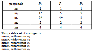 |
| |
|
6.3. The Existence of Stable Marriages
Let us prove that we do indeed get a stable matching from this algorithm.Theorem 11 Given n men and n women, there always exist a set of stable marriages.Proof: Suppose not. That is, suppose there was an unstable pair of marriages and defined earlier. Without loss of generality, let this pair be (m1, w1) and (m2, w2). Now this is an unstable pair of matchings so let m2 actually prefer w1. But then he would have proposed to her before proposing to his present wife w2. And w1 would not have rejected m2 since she prefers him to her current husband by definition of an unstable pair of marriages. Thus, this unstable situation would not result from the Stable Marriage Algorithm. So, the marriages cannot be unstable.
7. Timing Analysis and Comparison between the Algorithms
All three algorithms presented here run in polynomial time. Algorithm 1 works in  time. This means that for a balanced bipartite graph, we get a quartic running time,
  . To see this, consider the execution of the algorithm. Step 1 is done in time proportional to the size of the set X, and can be done at most that many times. Step 2 is performed at most n times, as this is the size of the set Y. Step 3 is also performed at most n times. Depending on the density of the input graph, the average running time of the algorithm might be lower. The space complexity of Algorithm 1 is
  [1, 13].Algorithm 2 works in quartic time,
  as well, in its original version[5]. However, there are implementations of this algorithm that work in cubic time,
  [6, 7]. The space complexity of Algorithm 2 is quadratic,
  as the size of the input is quadratic, and we do not use additional data structures.Algorithm 3 runs in quadratic time,
  in the worst case[8, 9]. It uses quadratic space for its input, and again as in Algorithm 2, the additional data structures can be maintained within quadratic space,
  . It is easy to see that at each step of the Marriage Algorithm the number of acceptances and the number of rejections is exactly n. However, there cannot be more than
  steps without acceptance, and at each step every man’s list becomes one position shorter.While this paper focuses on these three algorithms, there is a large body of research on matchings from both theoretical and algorithmic prospective. Many algorithms developed solve specific instances of matching problems[11, 12, 14, 15], and thus make us of the combinatorial structure of these problems. Thus, direct comparison between algorithms that solve matching problems might not be appropriate in some cases as they work under different inputassumptions/conditions.Implementational issues are not discussed in this paper, but there is significant research in this area, and literature that the reader may consult[6, 9, 10, 12].
ACKNOWLEDGEMENTS
Dr. Vassilev’s work is supported by NSERC Discovery Grant. Laura Huntington wants to acknowledge the help of Dr. Vassilev during the work on this paper.
References
| [1] | Ron Gould. Graph Theory, Chapter 7: Matchings and r-Factors, Benjamin/Cummings Publishing Co., Menlo Park, CA, 1988. |
| [2] | Daniel A. Marcus, Graph Theory: A Problem Oriented Approach, 1st Edition, MAA, 2011. |
| [3] | http://en.wikipedia.org/wiki/Vertex_(graph_theory) |
| [4] | http://en.wikipedia.org/wiki/Greedy_algorithm |
| [5] | Harold W. Kuhn. The Hungarian Method for the assignment problem, Naval Research Logistics Quarterly, 2:83–97, 1955. |
| [6] | James Munkres. Algorithms for the Assignment and Transportation Problems, Journal of the Society for Industrial and Applied Mathematics, 5(1):32–38, 1957. |
| [7] | Harold W. Kuhn. Variants of the Hungarian method for assignment problems, Naval Research Logistics Quarterly, 3: 253–258, 1956. |
| [8] | D. Gale and L. S. Shapley. College Admissions and the Stability of Marriage, American Mathematical Monthly 69, 9–14, 1962. |
| [9] | D. Gusfield and R. W. Irving. The Stable Marriage Problem: Structure and Algorithms. Cambridge, MA: MIT Press, 1989. |
| [10] | S. Skiena. Stable Marriages. §6.4.4 in Implementing Discrete Mathematics: Combinatorics and Graph Theory with Mathematica. Reading, MA: Addison-Wesley, 245–246, 1990. |
| [11] | Gerth S. Brodal, Loukas Georgiadis, Kristoffer A. Hansen and Irit Katriel. Dynamic Matchings in Convex Bipartite Graphs. Mathematical Foundations of Computer Science - MFCS, 406–417, 2007. |
| [12] | Takeaki Uno. Algorithms for Enumerating All Perfect, Maximum and Maximal Matchings in Bipartite Graphs. ISAAC 1997:92–101. |
| [13] | Uri Zwick. Lecture Notes on Maximum Matching in Bipartite and Non-Bipartite Graphs. December 2009. |
| [14] | J. E. Hopcroft and R. M. Karp. An algorithm for maximum matching in bipartite graphs, SIAM J. on Comp., Vol. 2: 225–231, 1973. |
| [15] | S. Micali and V.V.Vazirani. An Algorithm for Finding Maximum Matching in General Graphs. In Proceedings of 21st FOCS, 17–27, 1980. |
 Abstract
 Reference
 Full-Text PDF
 Full-Text HTML