Syed Tauhid Zuhori , Zahrul Jannat Peya , Firoz Mahmud
Department of Computer Science, Engineering, Rajshahi University of Engineering, Technology, 6204, Rajshahi
Correspondence to: Syed Tauhid Zuhori , Department of Computer Science, Engineering, Rajshahi University of Engineering, Technology, 6204, Rajshahi.
| Email: |  |
Copyright © 2012 Scientific & Academic Publishing. All Rights Reserved.
Abstract
The Multi-Depot Vehicle Routing Problem (MDVRP), an extension of classical VRP, is a NP-hard problem for simultaneously determining the routes for several vehicles from multiple depots to a set of customers with demand and then return to the same depot. Main goal of this thesis is to solve MDVRPSD in three phases. Firstly we’ve used nearest neighbour classification method for grouping the customers, then Sum of Subset method have been used for routing. Finally the routes are optimized using greedy method. The routes obtained using these methods are better for the vehicles considering demands of the customers. As an input we consider here some customers position, the depots position. Also the demand is initialized randomly. Here we solve the problem for 4 depots to 10 depots. The input customer ranges from 20 to 50. Then by using the three-phases the problem is solved for the input combinations. Actually the main target to solve this problem is to reduce the number of vehicles needed to serve the customers. We have to serve the customers of a definite route by a vehicle. So if the routes are minimized then number of needed vehicles is also minimized. The time is also an important issue. So the time is also measured for solving the whole problem with three-phases. So at the last part of the paper the performance is measured according to time for solving the problem and the number of vehicle needed for each of the problem.
Keywords:
Multi-Depot Vehicle Routing Problem, Sum of Subset, Greedy Method
Cite this paper:
Syed Tauhid Zuhori , Zahrul Jannat Peya , Firoz Mahmud , "A Novel Three-Phase Approach for Solving Multi-Depot Vehicle Routing Problem with Stochastic Demand", Algorithms Research , Vol. 1 No. 4, 2012, pp. 15-19. doi: 10.5923/j.algorithms.20120104.01.
1. Introduction
Typical Vehicle Routing Problem means determining routes for several vehicles from a depot to a number of customers and then returning to the depot.Since the problem is related with single depot, the VRP is also named Single-depot VRP. Single-depot VRPs are not suitable for practical situations. VRPs with more than one depot are known as Multi-depot Vehicle Routing Problem[1]. Our topics are Multi-depot Vehicle Routing Problem with Stochastic Demand. Here the customers are characterized by their own demand. The customers' demands are stochastic variables, on which only the probability distribution for each customer is assumed known at the time of planning, so that it is the expected total travel cost which is subjected to minimization[2].Nearest-neighbour classifiers are very simple to design, and often equal or exceed in accuracy much more complicated classification methods[3].For this reason we have used this classifier for grouping. Sum of Subset method first combines the demands of the customers for satisfying fixed constraints. This method finds routes at a faster rate thus providing computationally efficient solutions. Finally routes are scheduled using greedy method.In the figure we see that there are two depots and 9 customers. Every customer has its own number and also there is a demand with them. Three vehicles are needed here for serving the nine customers from the two depots. The first vehicle (a bus) serves the customer 1, 2 and 3 and it starts from depot A. The second vehicle (a racing car) serves the customer 7, 8 and 9 and it starts from depot B. The third vehicle (a racing car) serves the customer 4,5 and 6 and it also starts from depot B.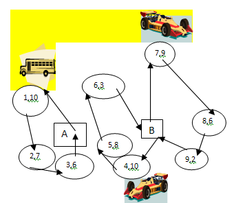 | Figure 1. An example of MDVRP with three vehicles, 9 customers with demands and 2 depots |
2. Literature Survey
In 1959, Dantzig and Ramser first introduced vehicle routing problem[6]. Wu et Al., reports a simulated annealing (SA) heuristic for solving the multi-depot location routing problem (MDLRP)[7]. Giosa et Al.[8], developed a “cluster first, route second” strategy for the MDVRP with Time Windows (MDVRPTW), an extension of the MDVRP. This can be shown by a table:| Table 1. Related work of MDVRPSD |
| | 1964 | Clarke and Wright developed a heuristic solution method named savings method and was the first algorithm that became widely used[2] | | 1969 | Tillman first addresses the VRPSD as a modification of the savings method | | 1986 | Reviews of work on the VRPSD are provided by Dror and Trudeau | | 19891996 | Dror et al. and Gendreau et al. Stewart and Golden presented three models for the VRPSD[2] | | 1992 | Laporte et al. introduced the VRP with stochastic travel and service times[2]. |
|
|
3. Methodology
We’ve used three independent methods to solve MDVRPSD.
3.1. Input
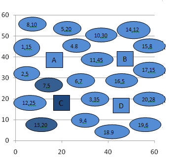
Figure2 indicates the initial customers and depot Locations. The circles indicate the customers (20 customers) and the rectangles indicate the depot locations (4 depots). The numbers associated with each customer denote the demands of the customers.We can also represent the figure 2(the input) in a table.| Table 2. Customers with corresponding demand |
| | Customer Number | Demand of the customer | | 1 | 15 | | 2 | 5 | | 3 | 35 | | 4 | 8 | | 5 | 20 | | 6 | 7 | | 7 | 5 | | 8 | 10 | | 9 | 4 | | 10 | 30 | | 11 | 45 | | 12 | 25 | | 13 | 20 | | 14 | 12 | | 15 | 8 | | 16 | 5 | | 17 | 15 | | 18 | 9 | | 19 | 6 | | 20 | 28 |
|
|
 | Figure 2. Initial customers and depot locations |
3.2. Nearest Neighbor Method
Nearest Neighbour technique makes a decision based on the shortest distance to the neighbouring class samples[5]. I have used this technique to assign the customers to their nearest depot. This process of assigning is called grouping.For measuring distance in Nearest Neighbour method I have used the following Euclidean formula[1]: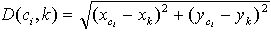 | (1) |
Here, ci = ith customer, k=depotAfter measuring distance the customers are assigned according to the following formula:-If D(ci ,A) < D(ci ,B), then customer ci is assigned to depot A- If D(ci ,A) > D(ci ,B), then customer ci is assigned to depot B-If D(ci ,A) = D(ci ,B), then customer ci is assigned to a depot chosen arbitrarily between A and B.After grouping I’ve got the following result: Here for example in the input figure1 the distance from customer 6 to depot A is 16.12 and the distance to depot D is 15.62.As distance to D is minimum,6 is assigned to depot D(Figure 1). In this way all other customers are assigned.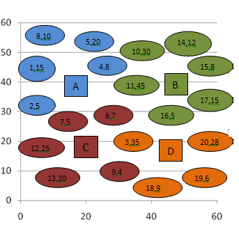 | Figure 3. After grouping using Nearest Neighbour method |
We can also represent the result shown in figure 3 in a table.| Table 3. Customers with corresponding depots after grouping |
| | Depot | Customer Number | Demand | | A | 1 | 15 | | 2 | 5 | | 4 | 8 | | 5 | 20 | | 8 | 10 | | B | 10 | 30 | | 11 | 45 | | 16 | 5 | | 17 | 15 | | 15 | 8 | | 14 | 12 | | C | 6 | 7 | | 7 | 5 | | 9 | 4 | | 12 | 25 | | 13 | 20 | | D | 3 | 35 | | 18 | 9 | | 19 | 6 | | 20 | 28 |
|
|
3.3. Sum of Subsets
Suppose we are given n distinct positive numbers (usually called weights). We desire to find all combinations of these numbers whose sums are m. This is called the sum of subsets problem[4].In our approach weights are considered as wi.Here 1≤i≤n.And denotes the demands of the customers. The value of m is given 50. After grouping we’ve used sum of subsets for determining the routes. In this case following flowchart is used.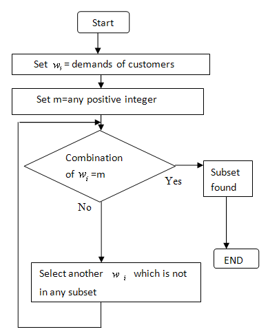 | Figure 4. Flow Chart of Sum of Subset Approach |
Here when combinations of wi i.e. demands of customers sum to 50 then we get a subset and it is the route. So the customers whose demands sum to 50 are linked to one route. Otherwise we try to make another subset with the rest customer’s demands. If no other subset is found then the rest customers are linked to an individual route.The result of applying Sum of Subset is shown in figure 4.Here in depot A (figure 5) the sum of the demands of the customers 1, 2, 8 and 5 is 50.The value of m is also 50.So we get a subset here. For this reason these customers are linked to one route. In depot A there is another customer i.e. customer 4.Demand of customer 4 is 8. It is not possible to get another subset here. A new vehicle is used to service customer 4.In this way other routes are determined.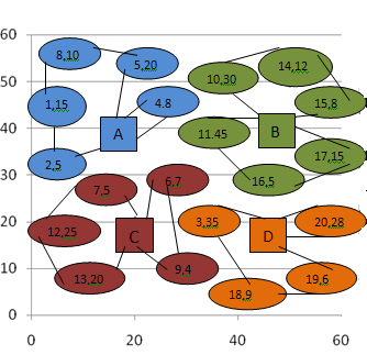 | Figure 5. Route obtained using Sum of Subset approach |
The result is shown in the table.| Table 4. Assignment of customers to depots using sum of subsets |
| | Depot | Routes | Vehicles | | A(11,40) | A-2-1-8-5-A | 2 | | A-4-A | | B(45,40) | B-10-14-15-B | 3 | | B-11-16-B | | B-17-B | | C(15,20) | C-13-12-7-C | 2 | | C-6-9-C | | D(45,20) | D-3-18-19-D | 2 | | D-20-D |
|
|
3.4. Greedy Method
Greedy method is the most straightforward design technique. This method suggests that one can devise an algorithm that works in stages, considering one input at a time. At each stage, a decision is made that appears to be the best (under some constraints) at the time[4]. In this case we have used the following flowchart:Here in depot A customer 1 is the closest node. So cost to customer 1 is minimum. The visit starts from customer 1.Then find another customer that is closer to customer 1.That customer is customer 2.So the vehicle goes to customer 2 from customer 1.The next customer is customer 4.At this position total demand is 28. So customer 5 can be included in the trip. But customer 8 can’t be included because that breaks the constraint. Customer 8 is serviced by a new trip.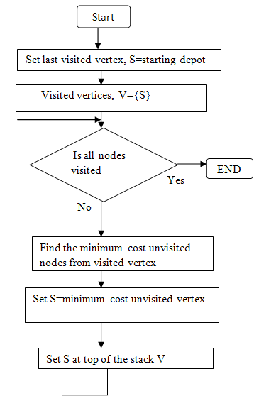 | Figure 6. Flow Chart of Greedy Method |
In this way all other routes are determined.| Table 5. Assignment of customers to depots using Greedy method |
| | Depot | Routes | | A(11,40) | A-1-2-4-5-A | | A-8-A | | B(45,40) | B-11-16-B | | B-17-15-14-B | | B-10-B | | C(15,20) | C-6-7-12-C | | C-13-9-C | | D(45,20) | D-3-18-D | | D-19-20-D |
|
|
4. Result Analysis
This section describes computational experiments carried out to investigate the performance of the proposed methods. Finding out routes using these methods is extremely easy for customization on similar problems.Here we solve the problem for 4 to 10 depots and the numbers of customers are also increased. The numbers of customers ranges from 20 to 50. We find the numbers of vehicle needed and also the time to solve the problem in second. The following table indicates the result.| Table 6. Number of vehicle needed and the time for each problem set |
| | Number of Customer | Number of Depot | Number of vehicle needed | Time to solve the problem(in sec) | | 20 | 4 | 9 | 0.5268 | | 25 | 5 | 13 | 0.8651 | | 30 | 6 | 17 | 1.2354 | | 35 | 7 | 20 | 1.8569 | | 40 | 8 | 22 | 2.2145 | | 45 | 9 | 24 | 2.3698 | | 50 | 10 | 27 | 2.8658 |
|
|
The following figures (figure 7 and figure 8) represent the result in a graph. The first graph shows the number of vehicle needed and the second graph shows the time required to solve the problem.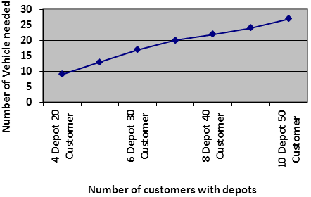 | Figure 7. The number of vehicles needed for each problem |
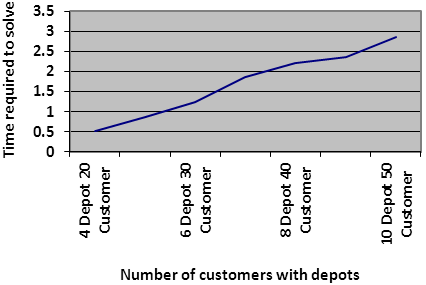 | Figure 8. The number of vehicles needed for each problem |
5. Scope and Limitations
We use the proposed methods to solve at least 10 depots and 50 customers There are some limitations of the methods. The three methods work statically rather than dynamically. The number of vehicle is minimum but time required for solving the problem is higher when the numbers of customers and depots are increased. Because the sum of subset is a backtracking method.
6. Summary and Conclusions
The main problem was to find routes of Multiple Depot Vehicle Routing Problem with Stochastic Demand. We first grouped the customers using nearest neighbor method. Then sum of subset method was applied in the grouped customers and routes were obtained. But in this method there was no indication for which customer will be serviced first. For this reason greedy method was applied.In future we intend to solve the problem dynamically. We will try to service large number of customers (such as 500 to 1000 customers).
References
| [1] | Surekha P. and Dr. S .Sumathi , “Solution To Multi-Depot Vehicle Routing Problem Using Genetic Algorithms”, Journal of Algorithm Optimization-August,2011, Pages 118-131. |
| [2] | Graham K Rand, “The life and times of the Savings Method for Vehicle Routing Problems”, International Journal of Operational Research,October-2009, Pages 132-135. |
| [3] | Neural Networks, Fuzzy Logic and Genetic Algorithms by S. Rajasekaran and C. A. Vijayalakshmi Pal, Chapter 2, Pages 29-30. |
| [4] | Fundamentals of Computer Algorithms by Ellis Horowitz,Sartaj Sahni and Sanguthevar Rajasekaran, Chapter 7, Pages 341-357. |
| [5] | Neural Computing; An Introduction by R Beale and T Jackson, Chapter 2, Page 20. |
| [6] | Aslaug Soley Bjarnadottir, “Solving the Vehicle Routing Problem with Genetic Algorithms”, International Journal of Electrical and Computer Engineering-April 2004, pages 23-27. |
| [7] | T. H. Wu, C. Low, and J. W. Bai, "Heuristic solutions to multi-depot location-routing problem," Computers & Operations Research, vol. 29, pp. 1393–1415, 2002. |
| [8] | I. D. Giosa, I. L. Tansini, and I. O. Viera, "New assignment algorithms for the multi-depot vehicle routing problem," Journal of the Operational Research Society, vol. 53, pp. 977-984, 2002. |
 Abstract
 Reference
 Full-Text PDF
 Full-Text HTML