Joy Dutta 1, Soubhik Chakraborty 2, Mita Pal 2
1Department of Computer Science & Engineering, B.I.T. Mesra, Ranchi, 835215, India
2Department of Applied Mathematics, B.I.T. Mesra, Ranchi, 835215, India
Correspondence to: Soubhik Chakraborty , Department of Applied Mathematics, B.I.T. Mesra, Ranchi, 835215, India.
| Email: |  |
Copyright © 2012 Scientific & Academic Publishing. All Rights Reserved.
Abstract
The present work aims to study the behavior of singleton sort algorithm for normal distribution inputs with a focus on parameterized complexity. Statistical bound estimates are obtained by running computer experiments working directly on time. It is found, using factorial experiments, that the parameters of normal distribution ( mean and standard deviation) along with the input size are all significant statistically both individually as well as interactively.
Keywords:
Singleton Sort, Parameterized Complexity, Factorial Experiments, Computer Experiments, Average Complexity
1. Introduction
The present paper examines the behavior of singleton sort algorithm for normal distribution inputs. The focus is on parameterized complexity where other parameters in addition to the input size n are useful in explaining the complexity more precisely; these “other parameters” here refer to the parameters of the input probability distribution. We use factorial experiments where n observations to be sorted come independently from normal (m, s) distribution. To study the individual effects of number of sorting elements (n), normal distribution parameters (m, s), as well as their interaction effects on the average sorting time, a 3-cube factorial experiment is conducted with 3 levels for each of the factors n, m and s. Here m and s stands for “mu” and “sigma”, the two population parameters representing the mean and standard deviation for normal distribution respectively. For brevity in typing, we have avoided the symbols µ (mu) and σ (sigma) that we use generally. In an earlier work Chakraborty and Dutta [1] have shown how Singleton sort is sensitive to parameters of the input probability distribution. But the interaction of these parameters was not investigated. For a comprehensive literature on sorting, we refer to Knuth[2]. For theoretical analysis on sorting with special emphasis on input distribution, see Mahmoud [3]. For computer experiments, including factorial experiments used therein, see Fang, Li and Sudjianto[4]. The first systematic work in parameterized complexity is credited to and Fellows[5]. Before moving to the main experimental findings we will discuss about singleton sort algorithm.Singleton sort algorithm is a modified and improved version of Hoare’s quick sort algorithm. It was introduced by R. C. Singleton in 1969 [6] in which he suggested the median of three methods for choosing the pivot. One way of choosing the pivot would be to select the three elements from the left, middle and right of the array. The three elements are then sorted and placed back into the same positions in the array. The pivot is the median of these three elements. A C++ implementation for the quick sort algorithm which employs the median of three methods can be found in Chakraborty and Dutta [1].
2. Empirical Results and Discussion
Assuming the sorting elements follow normal distribution (m, s), n independent normal (m, s) variates are obtained by simulation (using Box-Muller transformation [7]) and kept in an array before sorting. Table 1 below gives the average sorting time in seconds over 100 trials for different values of s when m and n are fixed at 10 and 50,000 respectively and s varied from 2 to 12 in the interval of 2 . The graphical plot is shown in Fig 1.| Table 1. Average sorting time for different value of s when n=50,000 and m=10 |
| | s | Avg sort time in seconds | | 2 | 0.01706 | | 4 | 0.01185 | | 6 | 0.01592 | | 8 | 0.01261 | | 10 | 0.01266 | | 12 | 0.01933 |
|
|
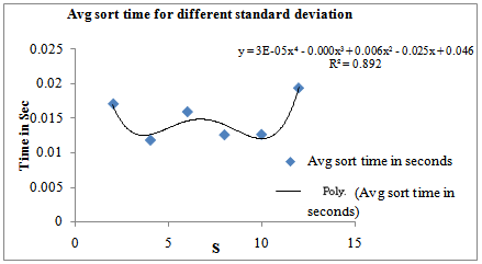 | Figure 1. Average time for different standard deviation, s when n=50000 and m=10: Fourth degree polynomial fitting |
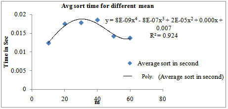 | Figure 2. Average time for different values of m when n=50000 and s=2: Fourth degree polynomial fitting |
| Table 2. Average sorting time for different values of m when n=50,000 and s=10 |
| | m | Average sort in second | | 10 | 0.01237 | | 20 | 0.01748 | | 30 | 0.0178 | | 40 | 0.01853 | | 50 | 0.0142 | | 60 | 0.01371 |
|
|
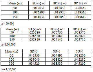
Table 3. Data for 3-cube factorial experiment for Singleton sort with normal distribution inputs
 |
| |
|
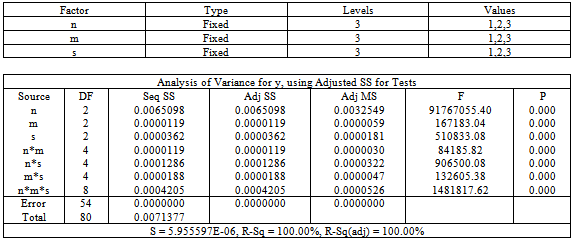
From Table 1and Fig 1, we get average sorting time yavg(s) = Oemp(s4). Average sorting time clearly depends on the parameter s of normal distribution and a polynomial of order four seems to be adequate to describe the average sorting time in terms of s when n and m are fixed. It is important to note here that empirical O, written as O with a subscript emp, is actually a statistical bound estimate. This is because it is obtained by directly working on time in which time of all operations, including repetitions, are collectively taken and mixed (added). In other words, we regard an operation’s time as its weight. This weight is not fixed and depends on the operation type, the system and even the operands. A weight based bound is a statistical bound and differs from the traditional count based mathematical bounds which are also operation specific. Statistical bounds are ideal for average case analysis for complex codes where it is difficult to detect the pivotal operation for applying mathematical expectation. Also the probability distribution over which expectation is taken may not be realistic over the problem domain. Which may be verified easily by running computer experiments. See Chakraborty and Sourabh [8], [9] by the same authors and the discussion in [1].In the next experiment we have varied m from 10 to 60 in the interval of 10 and kept s and n constant. Table 2 and the corresponding graph given in Fig 2 are noteworthy.Table 4. Result of 3-cube factorial experiment on Singleton Sort algorithm General Linear Model: y versus n, m, s
 |
| |
|
Results: From above, we get average sort time yavg(m) = Oemp(m4). Average sorting time clearly depends on the parameter m of normal distribution and a polynomial of order four is adequate to describe the average sorting time in terms of m when n and s are fixed. Since sorting time always depends on the number of sorting elements n, we conclude that, for singleton sort with n independent normal (m, s) inputs, all the parameters n, m and s are important in explaining the complexity. The question of importance is: Are their interactions also significant? This question is addressed next. With three parameters n, m and s, there can be three two factor interactions namely n *m, m * s and n * s and one three factor interaction n *m *s.Factorial Experiments : To investigate further into the matter, a 3-cube factorial experiment is conducted using n at 3 levels (50000, 100000, 150000) , m at 3 levels (50, 100, 150) and s at 3 levels (3, 5, 7) using MINITAB statistical package version 15. In our analysis, the three levels of n, m. s are coded as 1, 2, 3 respectively. Table 3 gives the data for factorial experiments to accomplish our study on parameterized complexity and Table 4 shows the results of the factorial experiments for singleton sort.It is evident from table 4 that Singleton sort is highly affected by the factors n, m and s both individually and interactively. When we consider the interaction effects, interestingly we find that all the interaction effects are significant. Particularly, the interaction factors n*s and n*m*s seem to be very highly significant.
3. Concluding Remarks
Three-cube factorial experiment conducted on singleton sort reveals that the parameters m and s of the normal input singularly as well as interactively are important besides the input size n for evaluating the time complexity more precisely. We obtained yavg(s) = Oemp(s4) and yavg(m) = Oemp(m4) for fixed n. It should be emphasized here that (i) the statistical approach is ideal for verifying the significance of interactions of input parameters in complexity analysis and (ii) a common objective in computer experiments is that we look for predictors that are cheap and efficient (see the seminal paper by Sacks. et. al.[10]). This is what empirical O does.
References
| [1] | Chakraborty, S. and Dutta, J., An Empirical Study on Parameterized Complexity in Singleton Sort Algorithm, International Journal on Computational Sciences and Applications, Vol.2, No. 2, p.1-14, April 2012, |
| [2] | Knuth, D. E., The Art of Computer Programming,Vol. 3: Sorting and Searching, Pearson Education reprint, 2000. |
| [3] | Mahmoud, H., Sorting: a Distribution Theory, John Wiley & Sons, 2000 |
| [4] | Fang, K. T., Li, R. and Sudjianto, A., Design and Modeling of Computer Experiments, Chapman and Hall, 2006 |
| [5] | Downey, R. G. and Fellows, M. R., Parameterized Complexity, Springer, 1999 |
| [6] | Singleton, R. C. Algorithm 347: An Efficient Algorithm for Sorting with Minimal Storage, Comm. ACM, 12, 3, p.185-187, 1969 |
| [7] | Kennedy, W. and J. Gentle, Statistical Computing, Marcel Dekker Inc, 1980 |
| [8] | Chakraborty, S. and Sourabh, S. K., A Computer Experiment Oriented Approach to Algorithmic Complexity, Lambert Academic Publishing, 2010 |
| [9] | Chakraborty, S. and Sourabh, S. K., On Why an Algorithmic Time Complexity Measure can be System Invariant rather than System Independent, Applied Math. and Compu, Vol. 190(1), p. 195-204, 2007 |
| [10] | Sacks, J., W. Welch, T. Mitchell and H. Wynn, Design and Analysis of Computer Experiments, Statistical Science, vol. 4(4), p. 409-423, 1989 |
 Abstract
 Reference
 Full-Text PDF
 Full-Text HTML