-
Paper Information
- Paper Submission
-
Journal Information
- About This Journal
- Editorial Board
- Current Issue
- Archive
- Author Guidelines
- Contact Us
American Journal of Signal Processing
p-ISSN: 2165-9354 e-ISSN: 2165-9362
2025; 13(1): 1-16
doi:10.5923/j.ajsp.20251301.01
Received: Jul. 10, 2025; Accepted: Aug. 3, 2025; Published: Aug. 8, 2025

Machine Learning-Based Fault Diagnosis and Characterization System for Power-Generating Sets Using Customized Fault Audio Dataset
 Abstract
 Reference
 Full-Text PDF
 Full-text HTML
Ekerette Ibanga, Kingsley Udofia, Kufre Udofia, Unwana Iwok, Emmanuel Ogungbemi
Department of Electrical and Electronics Engineering, Faculty of Engineering, University of Uyo, Uyo, Nigeria
Correspondence to: Ekerette Ibanga, Department of Electrical and Electronics Engineering, Faculty of Engineering, University of Uyo, Uyo, Nigeria.
| Email: |  |
Copyright © 2025 The Author(s). Published by Scientific & Academic Publishing.
This work is licensed under the Creative Commons Attribution International License (CC BY).
http://creativecommons.org/licenses/by/4.0/

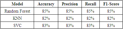
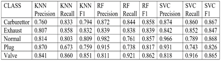
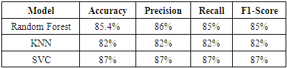
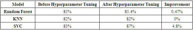
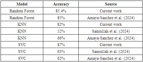
The growing dependency on stable power supply has made unexpected downtime a dreaded event. Research in Signal processing and machine learning techniques have become hot areas for the diagnosis of faults in power-generating systems due to their advantages, which include fast diagnosis, high detection accuracy, good generalization, and low cost. The focus of this work is to use a customized dataset to develop a machine learning-based system for fault diagnosis in selected domestic power-generating sets. The approach analyses the unique sound patterns associated with each fault type for twenty-five 5kVA generators under five distinct operational conditions: carburetor fault, exhaust blockage, loose valve, weak Plug, and normal. Signals were pre-processed, normalized and discriminative features extracted and converted to numerical representations of the fault audio patterns. The Support Vector Machines (SVC), random forest, and K-Nearest Neighbours (KNN) supervised machine learning algorithms were trained on the annotated feature datasets and classified for the type of fault. The performance of each model was evaluated using key performance metrics, including accuracy, precision, recall, and F1-score, with k-fold cross-validation (k=10) to ensure generalizability, as well as a confusion matrix to derive performance measures for each condition. Before hyper-parameter tuning, these models achieved accuracies of 85%, 82%, and 83%, respectively. Notably, SVC demonstrated a significant improvement post-tuning, with accuracy increasing by 4.8% to 87%. In contrast, Random Forest showed a slight increase of 0.47%, while KNN showed no improvement. The results from the confusion matrices showed better classification performance for SVC compared to KNN and Random Forest. This indicates that SVC is most suitable for real-time deployment in fault diagnosis of generator systems based on audio signals.
Keywords: Machine learning, Fault diagnosis, Signal processing, Feature extraction, Power generator faults
Cite this paper: Ekerette Ibanga, Kingsley Udofia, Kufre Udofia, Unwana Iwok, Emmanuel Ogungbemi, Machine Learning-Based Fault Diagnosis and Characterization System for Power-Generating Sets Using Customized Fault Audio Dataset, American Journal of Signal Processing, Vol. 13 No. 1, 2025, pp. 1-16. doi: 10.5923/j.ajsp.20251301.01.
Article Outline
1. Introduction
- Power-generating systems, which include equipment such as diesel or petrol generators, wind turbines, hydroelectric generators, and solar power inverters, are essential for the continuous supply of electricity, supporting a wide range of applications from large-scale industrial operations to individual households. With the demand for stable electricity, it becomes necessary to operate these systems online. Early and effective fault diagnoses can mitigate the risks associated with power system failures [1] [2] and ensure optimal performance. A system that automatically collects signal data processes it, classifies the data, and diagnoses the fault can provide security in the surveillance of critical assets, such as electrical substations and industrial scenarios, reduce downtime of machines, decrease maintenance costs, and avoid devastating accidents [3]. The power generator comprises six subsystems: the stator winding, rotor winding, stator core, mechanical components, cooling system, and excitation system. Faults can be mechanical wear and component degradation arising from worn-out bearings, misaligned shafts, or lubrication failure, electrical imbalances such as voltage imbalances, short-circuit faults, or faults in the alternator, thermal stresses, which typically manifest as overheating affecting critical components such as turbines, engines, or cooling systems. To avoid costly downtime, extensive repairs, and, in extreme cases, system failure, fault diagnosis systems should be implemented promptly [4] [5] to determine which subsystem is affected and which type of failure is present. Fault diagnosis in power-generating systems has historically progressed from manual inspections and simple monitoring techniques to traditional methods, including vibration analysis and thermal imaging, which have high installation costs and are affected by surrounding equipment, leading to poor diagnostic accuracy and reliability [6]. These traditional methods were the primary source of signal capture for data-driven methodologies, which were prone to human error and inefficiency, particularly in complex systems operating under dynamic conditions, resulting in delayed fault detection and reactive maintenance. This led to an increased risk of catastrophic failures and extended downtime of critical equipment [7] [8]. However, sound sensors that capture acoustic sound signals are becoming increasingly popular for fault diagnosis over conventional vibration sensors [9].Current mechanical fault diagnosis technology is based on the analysis of signals, such as vibration signals [10], force signals, and audio signals. This is because acoustic sensor-based monitoring is an emerging area of interest due to its ability to accurately capture fault signatures and improve the detection accuracy of system anomalies [9]. This fault diagnosis approach utilizes audio-digital processing and transformation techniques to extract valuable information about the system's internal state from the unique acoustic signatures generated by distinct faults. These signals, generated by machinery during both normal and faulty operations, are captured and analyzed to identify specific issues within the system. This signal-based fault diagnosis method offers benefits such as high precision, low cost, great generalizability, and non-contact measurement. Examples of audio signal analysis methods include Fourier Transform, wavelet analysis [11], and Short-Time Fourier Transform (STFT) [12] [2]. In addition to signal processing techniques, the application of machine learning algorithms, including Support Vector Machines (SVMs) and Artificial Neural Networks (ANNs) [13], as well as tree-based classifiers, has revolutionized the diagnosis of faults in machinery.The use of audio signal processing combined with machine learning for fault diagnosis introduces several novel aspects compared to traditional methods (e.g., vibration analysis, thermal imaging, or manual inspection). It provides non-contact, non-intrusive monitoring with less expensive and minimal hardware. Fault patterns are detected early and in real-time by the models, thus improving preventive maintenance. It is computationally inexpensive and is suitable for remote, rural, or developing regions. The customized audio dataset, tailored to specific power-generating systems, introduces domain-specific intelligence and enables more accurate and context-aware models, rather than generalized diagnostic systems. The introduction of additional sensor capabilities enables a hybrid system for enhanced fault diagnosis. Collecting data is necessary to integrate machine learning algorithms into fault diagnosis, enabling fast and accurate real-time fault detection, which translates to reduced downtime. [14] However, it can be challenging to distinguish between primary data and noise, as the acquired data often contains noise from the surrounding environment that is processed in subsequent stages. Identifying fault issues in power-generating sets is a challenge in modelling where no prior knowledge of the unique characteristics of failure conditions exists for the machine case study. This can ultimately degrade the model's performance by yielding inaccurate fault diagnosis. [9]. Traditional fault diagnosis methods are plagued by problems, including time-consuming practices, labor-intensive processes, and susceptibility to errors, leading to prolonged downtime and increased operational costs.This research aims to address these challenges by developing a robust fault diagnosis system that integrates audio processing with machine learning techniques to enable the real-time identification and categorization of faults in power-generating systems. The contributions of this work are as follows:-i. Provides statistical data associated with each type of fault for the selected power-generating sets.ii. Pre-process and annotate recorded audio data from the selected power-generating systems under diverse fault conditions.iii. Leveraging audio signal processing tools such as mel-frequency cepstral coefficients (MFCC), continuous wavelet transform (CWT), and short-time Fourier transform (STFT) for the extraction of features that capture the unique acoustic signatures associated with selected fault conditions.iv. To utilize data-driven machine learning methods, such as KNN, SVC, and Random Forest, in fault classification and diagnosis for select power-generating systems.v. To evaluate the performance of the machine learning models in fault diagnosis of the selected power-generating sets.vi. To conduct real-time testing of the developed fault detection and characterization system under real-world operating conditions.This study focuses on audio samples recorded from 25 5kVA petrol-power generating systems under controlled settings and with respect to four fault conditions compared to normal conditions. The fault conditions considered include carburetor issues, exhaust problems, valve malfunctions, spark plug faults, and normal operational states. This scope reduces the system's applicability to a broader spectrum of potential faults commonly found in power-generating sets. The system relies solely on audio signals for fault detection. Hence, faults that do not produce distinctive acoustic signatures or are masked by ambient noise may go undetected. The system is designed for closed-set fault classification, where all possible fault conditions are pre-defined and may struggle with open-set fault diagnosis.
2. Literature Review
- Fault diagnosis in power-generating systems involves identifying and characterizing fault issues and is critical to ensuring the reliable operation of power-generating sets. A stable power supply is essential in various sectors because faults degrade efficiency, causing increased fuel consumption, reduced output, and higher operational costs [15] [16]. Predictive maintenance (PdM) techniques like audio signal analysis and machine learning enable real-time identification of anomalies, allowing timely interventions [17]. The advantage of this approach is that it reduces maintenance costs, minimises downtime, and extends equipment lifespan [18]. Audio signal processing addresses some limitations of traditional diagnostic methods like vibration analysis [19] [20] or infrared thermography [21] [22] that require specialized sensors and direct access to machinery. Audio-based methods utilise non-intrusive microphones to capture sound emissions from equipment and are particularly useful in hazardous areas [23] [24]. Audio signals obtained from acoustic emission-based techniques have emerged as effective tools for diagnosing faults in power-generating systems [25] [26]. These sound signals originating from various mechanical activities, such as friction, impacts, and material deformation, which occur during the operation of power-generating sets, are used to identify and characterize mechanical faults like bearing wear, misalignments, cracks, and rotor imbalance [27]. Other common faults associated with generator sets are faults associated with the Carburetor [28] [29], valves [30], plugs, and exhaust systems. Audio signal processing can be incorporated into machine learning (ML) for automating fault characterization by enabling the detection of patterns in complex datasets. ML algorithms (Fast Fourier Transform (FFT), Support Vector Machines (SVM) [31], Decision Trees [32] [33], K-Nearest Neighbors (KNN) [34] [35], [36], or Neural Networks [37], [38], [39] can process volumes of data, learn and distinguish between normal and faulty conditions [40] [41] This integration further strengthens the diagnostic process by leveraging advanced feature extraction techniques such as temporal and spectral feature extraction techniques, Mel-Frequency Cepstral Coefficients techniques, time-localized Fourier transforms (STFT), auditory-inspired cepstral descriptors (GFCCs), and wavelet transforms. The key features of audio signals that are relevant for fault detection include frequency, amplitude, and phase [42]. Each of these features provides insights into different aspects of the machinery's behaviour and can be crucial for identifying faults in their early stages.A. Related WorksThe robust capacity for feature extraction and classification of linear and non-linear relationships using machine learning (ML) algorithms has led to several proposals for the use of artificial intelligence (AI) methods in fault diagnosis. ML algorithms provide high flexibility and fault diagnosis performance [43]. ML algorithms such artificial neural networks (ANN) [44]; [45]; [46], decision tree (DT) [47], Bayes network [48], extreme learning machine (ELM) [49], K-nearest neighbors (KNN) [50] [51], linear discriminant analysis (LDA) [52], logistic regression (LR) [53], support vector machine (SVM) have been used for faults diagnosis and detection in transformers transformer [54].Numerous machine learning application have been geared towards fault diagnosis in ship or aircraft and in diesel generators such as ship diesel generator diagnosis using fuzzy logic [55], diesel generator diagnosis and fault detection in wind turbines using deep learning [56] [57], and synchronous generator fault diagnosis using ANN [58] [59].[60] carried out a comparative analysis of three (3) machine learning models (Simple, ensemble, and gradient boost) developed for diagnosing faults in power generators using a customized generator fault database (GFDB). The data was pre-processed and hyperparameters selected while the performance of the models was evaluated using key performance metrics including accuracy, precision, recall, and F1-Score. Their findings revealed that the gradient boost demonstrated superior detection of the class 3 and class 4 faults. Although the GB model showed excellent overall performance, it particularly misclassified class 1 and class 2 faults. Comparing the confusion matrices for both GB and decision tree (DT) models showed that GB achieved high accuracy (≥80%) for most fault types. The major limitation of the study was associated with not identifying negative cases correctly (specificity) with each fault class. Also, the research categorized the faults in a general manner as catastrophic failures and specific fault types 0, 3, 4, and 5, creating a gap in understanding the root causes of the faults. Thus limiting effective maintenance and troubleshooting in power-generating sets. Also, the use of a curated dataset is another significant limitation of the study. The authors [61] proposed a system for machinery health monitoring during operation and an alert system for potential failures. The system was developed using noise signals collected from the electrical system of rotating machinery, such as electric motors, turbine generators, and bearing fault motors with microphones. The study demonstrates that mechanical faults in rotating machinery can be effectively diagnosed by analyzing the noise signals emitted in association with mechanical vibrations. The noise signal analysis focuses on vibration-induced noise signatures. The automated noise analysis system showed high efficacy in detecting abnormal conditions in machinery and providing early fault alarms. Additionally, the system offers the advantage of practical implementation without significantly increasing the size or power requirements of the monitored motors. While the system is effective in detecting faults, the study does not address fault classification, leaving the specific categorization of detected faults unexplored. A fault diagnosis system using Electrical Signature Analysis (ESA) for operational synchronous generators (SGs) dynamically integrated into the active power grid within bulk electric systems was explored [62]. This technique is employed for predictive maintenance to enhance SG protection and reliability. The electrical signals were processed and analyzed using the FFT algorithm to detect significant changes indicative of faults. The methodology was tailored for fault detection in wound-rotor synchronous generators (SGs), with an emphasis on current signature analysis (CSA) over voltage signatures. The study identified operational defects and anomalies, such as stator winding imbalances and rotor misalignment, through spectral signature analysis in the frequency domain. The results demonstrate ESA's effectiveness in condition monitoring and fault detection for SGs connected to power systems. The deployed prototype identified two faults: Interphase Short Circuit in the Stator Windings circuits detected through an imbalance in electrical patterns, and rotor misalignments identified through frequency patterns of the rotor. The findings validate ESA's potential for non-invasive predictive maintenance of SGs within interconnected power systems. However, the system was limited to fault diagnosis in SGs within bulk electric systems, suggesting the use of artificial intelligence techniques to enhance system automation and diagnostics. The proposed system by [63] utilized signal processing and machine learning to identify faults in induction motors, thereby mitigating industrial downtime and plant disturbances. MATLAB Simulink was used to generate the dataset for faults induced at different load conditions and severity levels. The 150,000 data points comprised variables encompassing electrical parameters (e.g., stator and rotor currents), active power consumption, rotational dynamics (slip, rotor angular velocity), and operational efficiency metrics (e.g., energy conversion efficiency). The experimental setup incorporated four distinct failure modes: conductive path interruption (open circuit), aberrant current pathways (short circuit), sustained overcurrent conditions (overload), and structural degradation of rotor elements (broken rotor bars). A fast Fourier transform (FFT) was used for feature extraction, and four classification algorithms—Decision Trees, Naïve Bayes, K-Nearest Neighbors (KNN), and Support Vector Classifier (SVC) — were employed for fault diagnosis. The system was not deployed in a real-world environment but was simulated in a MATLAB environment. The models were evaluated using key performance metrics, including predictive accuracy, sensitivity (also known as recall), and the F1 score. The results demonstrate that the Decision Tree algorithm had improved performance compared to the other models, achieving an accuracy of 92.1%. Naïve Bayes, KNN, and SVC achieved lower accuracies of 61.3%, 52%, and 63%, respectively.
3. Methodology
- This section outlines the materials used to implement this work and describes the method's structure. A combination of hardware and software resources was utilized to accomplish this task. The list of materials used is presented below. 1) A mobile phone of the following specification was used for audio data collection, capturing signals from 25 5kVA power-generating systems under various fault and normal conditions. Phone Performance Capabilities Brand: Infinix Smart 8; Operating System: Android 11(Go edition) with HIOS 7.6; Chipset: MediaTek 6762 Hello P22 (12nm); CPU: Octa-core 2.0GHz Cortex-A53; GPU: PowerVR GE8320.2) Laptop Specifications: HP, Windows 10 Pro, 11th Generation Intel® Core™ i5 processor, 16 GB memory; 256 GB SSD storage, 14″ diagonal FHD display, Intel® Iris® Xe Graphics for data processing, model training, and testing. 3) Jupyter Notebook Python software with a suite of specialized libraries including Scikit-learn, Librosa, Scipy, Spafe, Noise Reduce, and Pywavelets were used for audio signal processing, data pre-processing tools including Pandas and NumPy, Visualization tools like Matplotlib and Seaborn, feature extraction, noise reduction, and system development (Google Colab streamline experimentation). 4) System deployment was done using a Raspberry Pi 3 microcontroller, microphone sensors, communication modules (Wi-Fi), and an LCD module to implement and test the fault diagnosis system in real-world settings.A structured methodology was used to develop a fault diagnosis and characterization system for power generators, as shown in Fig. 1.
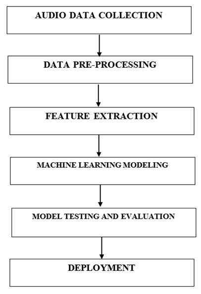 | Figure 1. Block Diagram of System Methodology |
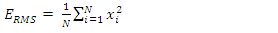 | (1) |
 denotes the discrete temporal instances of the acoustic waveform, and N signifies the cardinality of the sampled dataset under analysis.2) Zero Crossing Rate (ZCR): The Zero Crossing Rate (ZCR) is used to quantify the frequency of polarity transitions (positive to negative or vice versa) between consecutive waveform samples in an acoustic signal. A binary threshold function was used to output 1 (unity) when adjacent samples exhibit opposing polarities; otherwise, it outputs zero. These transitions provided insights into the noisiness and periodicity characteristics of the acoustic signals obtained. The Zero Crossing Rate (ZCR) was implemented using Equation 2.
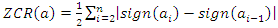 | (2) |
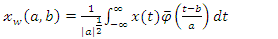 | (3) |
 represents the mother wavelet, a continuous, integrable function defined across both temporal and spectral domains,
  is the complex conjugate facilitating the generation of derived wavelet functions (daughter wavelets) through scaling
  and translation
  operations, and
  is the resulting wavelet coefficient represented as a scalogram. The scalogram output from Equation 3 is transformed using the Morlet wavelet as shown in Equation 4 into the time-frequency representation.
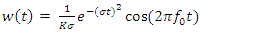 | (4) |
 is the Morlet wavelet function,
  is the centre frequency typically around 0.8125 in normalized units and bandwidth
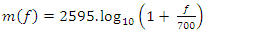
  . 4) Mel-Frequency Cepstral Coefficients: the mel-frequency cepstral coefficients (MFCCs) features were obtained first by applying pre-emphasis to the audio signal to amplify the energy of higher frequencies by adjusting the tilt of the spectrum. This step gives added robustness to our model because the energy content of higher frequency components of the generator audio is increased. The pre-emphasis is implemented using the general equation expressed in Equation 5.
 | (5) |
 is a dimensionless factor typically about 0.97 and x(t) the original signal.The commonly used Hamming window function was applied to each framed signal to ensure smooth transitions to zero at the ends, thereby reducing artifacts in time-frequency representations, minimizing spectral leakage, improving frequency accuracy, and producing cleaner spectrograms. This is usually done before frequency analysis.The Hamming window is expressed in Equation 6:
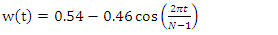 | (6) |
 and
and  is the lengthThe frequency spectrum of each windowed frame of the acoustic signal was obtained by applying the Fast Fourier Transform (FFT) to each windowed frame. The Fast Fourier Transform (FFT) is used to compute both the Discrete Fourier Transform (DFT) and its inverse. The DFT converts a time-domain signal into its frequency-domain representation by resolving it into sinusoidal components of varying frequencies. The FFT is implemented as shown in Equation 7.
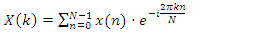 | (7) |
 represents the magnitude of the FFT.After applying the FFT to each windowed frame, we obtained the complex-valued frequency components. The absolute value of the FFT for the windowed frame is obtained as shown in Equation 8:
 | (8) |
 is the FFT of the windowed frame, and
  and
and  are the real and the imaginary components, respectively.The power distribution of each frequency component within each windowed frame is computed using the power spectrum and is presented in Equation 9.
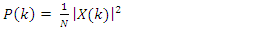 | (9) |
 | (10) |
 | (11) |
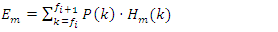
 is the energy in the
  Mel filter,
  is the power spectrum at frequency k, and
  is the Mel filter's magnitude response of the
  filter at frequency k.The log-transformed power spectrum undergoes conversion into cepstral coefficients using the Discrete Cosine Transform (DCT), which serves as a type of inverse Fourier transform to convert the log-power spectrum from the spectral to the cepstral domain. This stage effectively decorrelates the features to enhance their suitability for pattern recognition and machine learning models. This process leverages the mathematical properties of the cepstral domain to isolate independent signal components, optimizing discriminative performance in audio analysis applications. The DCT compresses the signal information into the first few coefficients, making the features more compact and easier to model. This is shown in Equation 12.
 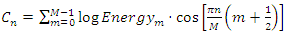 | (12) |
 denotes the n-th Mel-Frequency Cepstral Coefficient, capturing spectral characteristics in the cepstral domain, M represents the total number of triangular Mel-spaced filters applied to the power spectrum, and n defines the truncation limits for the cepstral coefficients,
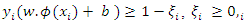
  uantifies the logarithmic energy output of the m-th Mel-frequency band, enhancing perceptual relevance.D. Machine Learning Algorithms (Model Training and Testing)The machine learning algorithms used in this work were the Support Vector Classifier (SVC), K-Nearest Neighbor (KNN), and Random Forest classifiers. The extracted features were split into a 70:30 ratio for training and testing the models, using a 10-fold cross-validation for model generalizability. The Support Vector Machine (SVM) is a discriminative supervised learning model efficient in high-dimensional feature spaces. Its kernel-driven transformations enable robust classification of both linearly and non-linearly separable data distributions. It utilizes kernel tricks to solve non-linear problems by mapping the input features into a higher-dimensional space, where a linear separation can be achieved. Some kernels include linear, polynomial, radial basis function (RBF), and sigmoid.
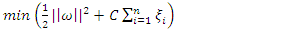 | (13) |
 Where
Where  represents kernel-induced feature space transformation,
  introduce flexibility by tolerating marginal classification errors, particularly for non-separable datasets, and
  governs the trade-off between maximizing the classifier's margin and penalizing misclassified instances, ensuring robustness to overfitting. The hyper-parameter tuning of the SVC model was achieved using the parameters – # Hyperparameter tuningsvc = SVC(probability=True)param_grid={'C':[1,10,100,1000],'gamma':[1,0.1,0.001,0.0001], 'kernel':['rbf']}grid = GridSearchCV(svc, param_grid, refit=True, verbose=3)grid.fit(X_train, y_train)print("Best Parameters:", grid.best_params_)print("Best Estimator:", grid.best_estimator_)The k-nearest neighbour's machine learning algorithm is a simple, effective, and instance-based non-parametric learning method used in this work for classification. This algorithm operates on the principle of similarity, leveraging the proximity of data points (measured by Euclidean distance) in a feature space to make predictions. The Euclidean distance metric used to quantify the similarity between instances is given in Equation 14.
 | (14) |
 | (15) |
 is the prediction of the b-th tree. The hyperparameter tuning phase of the random forest model was done using the parameters in the code –
 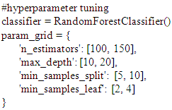 E. Evaluation Metrics of Fault Diagnosis The following are metrics used in evaluating the effectiveness of the fault diagnosis systems. 1) Accuracy (ACC)This metric represents the ratio of correctly diagnosed faults to the total number of diagnosis attempts.
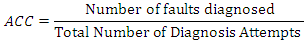 2) Precision (Positive Predictive Value)The precision metric measures the accuracy of positive diagnoses. It calculates the ratio of correctly diagnosed positive instances to the total number of instances diagnosed as positive. It protects the system from raising a false alarm.
 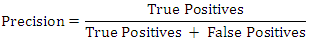 The precision metric says - out of the predicted fault cases, how many were actual faults?3) Recall (Sensitivity)Recall, which assesses the sensitivity of the system, was used to measure the proportion of actual positive instances that the system correctly diagnosed.
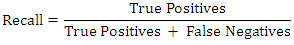 The recall metric says - out of all actual faults, how many did we correctly detect?4) F1-ScoreThe F1-score metric is suitable for an audio-based fault diagnosis system because it balances the detection of actual faults and the avoidance of false alarms, especially under imbalanced and high-risk conditions. F1-score is the harmonic mean of precision and recall. It provides a balance between these two metrics.
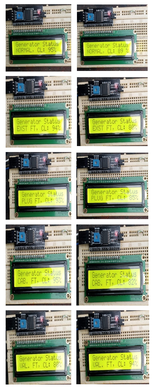
  Since fault data is often unbalanced, the F1-score serves as a means to penalize models that ignore the minority class (faults) in favor of the majority class (normal conditions). It also provides a single, interpretable metric for comparing model performance under different training or feature extraction conditions. The F1 score ranges from 0 to 1, with a value of 1 indicating perfect precision and recall.F. System DeploymentThe deployment design for this research, which enables the real-time classification of faults in power-generating systems based on audio signals, is illustrated in the block diagram of Figure 2. The system operates through the input stage, utilizing sound recording, the intermediary stage with signal processing, and the output stage, which involves user visualization. The system design is structured in such a manner that once it is powered on, it initiates a sequence of operations that involves capturing audio signals by recording, processing them through the machine learning model (signal processing and classification), and displaying the fault diagnoses (user interpretation) for the power-generating sets.
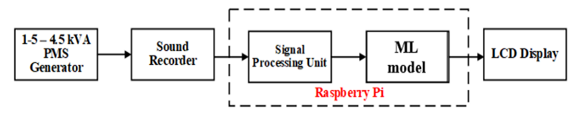 | Figure 2. Block Diagram of System Prototype |
4. Results and Discussion
- In this section, the results of the experiments carried out are presented and discussed under each subsection. A. Waveforms of Generator Audio Signals and Spectrograms.Fig. 3 shows the waveform visualizations of the generator audio signals. They exhibit distinct temporal characteristics and variations in amplitude and frequency patterns associated with different fault conditions. These waveforms were pre-processed, and features were extracted for model development and used for diagnosing generator faults. The spectral signatures, which show the distinct temporal characteristics and variations in amplitude and frequency patterns of the audio signals, are presented in Fig. 4.
 | Figure 3. Waveforms of Recorded Generator Audio Fault Signals |
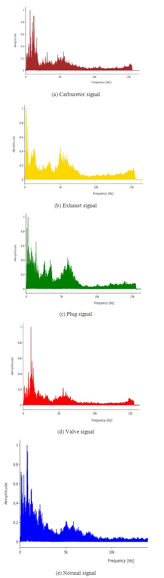 | Figure 4. Spectral Signatures of Recorded Generator Audio Fault Signals |
|
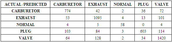
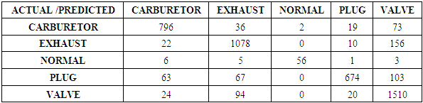
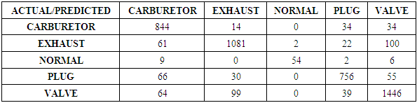
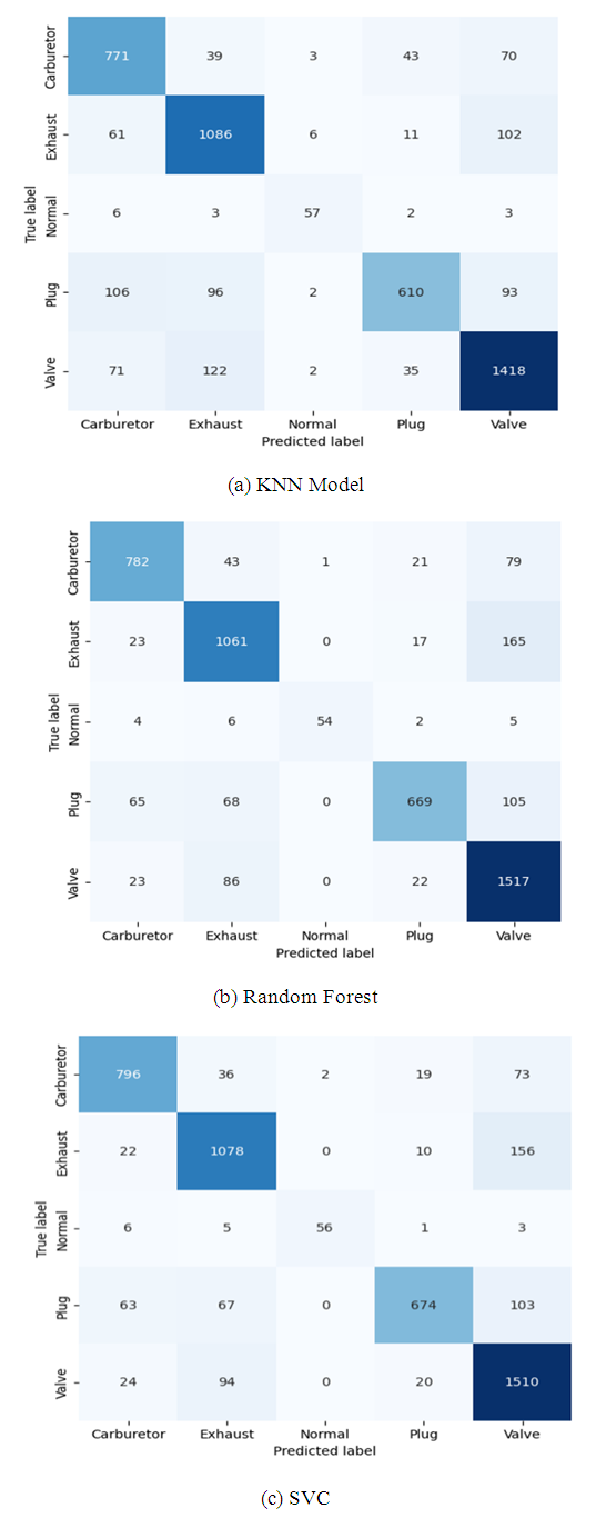 | Figure 5. Confusion Matrices for Machine Learning Models without Hyperparameter Tuning |
|
|
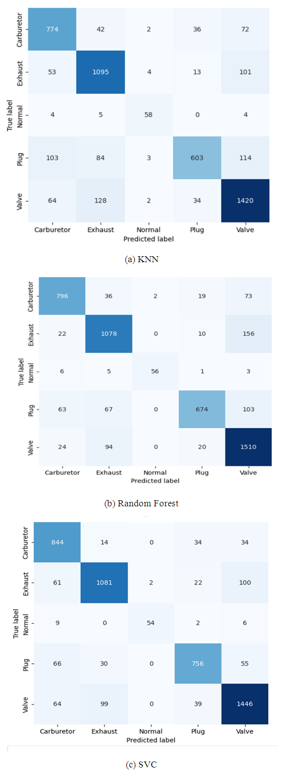 | Figure 6. Confusion Matrices for Machine Learning Models with Hyperparameter Tuning |
|
|
|
|
|
|
|
 | Figure 7. Accuracy Results of Different Faults Diagnoses for 2 Power Generators |
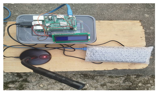 | Figure 8. Picture of System Prototype |
5. Conclusions and Recommendations
- In this work, experiments were carried out to develop and test three machine learning (3) models for the diagnosis and characterization of three (3) mechanical faults, one (1) electrical fault, and Normal operation for power-generating sets. The fault features were extracted from the audio signals of the customized dataset, which was collected from 25 5kVA petrol-powered generator sets. The results obtained from testing the models showed that the models performed better with hyper-parameter tuning, especially the SVC. The SVC model consistently performed better than the other two (2) models across most categories, as well as the external benchmarks used. This outstanding performance is made possible because SVC can handle high-dimensional audio signals by separating the classes using an optimal hyperplane. It also uses the appropriate kernel and bias versus variance balance parameters. It is less affected by noise and can model complex non-linear boundaries, unlike basic Random Forests. Suggestions for further workTo enhance the robustness of the fault detection system, future work could expand the dataset to include a broader range of fault conditions and generator types. A multi-modal fault diagnosis system can be created by combining acoustic signal processing with other sensor data, such as vibration and/or temperature data. This will provide more comprehensive information about generator behaviour under fault conditions.All the models performed better with hyper-parameter tuning which suggests that there is room for further optimization. In addition, more advanced models can be explored.In this work, the study was limited to twenty-five 5kVA generator set. For better generalizability, studies can be expanded to accommodate more generator types and brands. Our ML system was working well in controlled tests, however, more work investigating real-time deployment frameworks and edge-based solutions to assess feasibility and responsiveness in practical settings with respect to latency, actual hardware deployement and performance reliability under noisy real-world conditions. The scope of this work is in traditional machine learning models. Additional deep learning models (e.g., ANNs, CNNs or LSTMs) to compare performance against these and other classical ML algorithms can be explored especially for temporal and spectral audio features.