Dante C. Youla1, Fred Winter2
1New York University Tandon School of Engineering, United States
2Advanced Energy, United States
Correspondence to: Fred Winter, Advanced Energy, United States.
| Email: |  |
Copyright © 2020 The Author(s). Published by Scientific & Academic Publishing.
This work is licensed under the Creative Commons Attribution International License (CC BY).
http://creativecommons.org/licenses/by/4.0/

Abstract
Owing in part to the increasing importance of pulse width modulation (PWM) as an alternative analog communication technique for optical data links there has been a resurgence of interest in both new and traditional methods of analysis. Of the latter, the old pseudo-static approach is undoubtedly the simplest, although long considered by many to be only an approximation. One principal object of this paper is to prove that pseudo-static analysis is exact and explicit for natural ramp-intersective PWM and allows easy derivation of all pertinent time-domain formulas. As shown in detail by example, it then may be possible to carry out spectral and modulation-demodulation analysis in a straightforward physically insightful quantitative manner.
Keywords:
Ramp Intersective, PWM, Modulation, Demodulation, Spectral Analysis, Pseudo Static, Exact
Cite this paper: Dante C. Youla, Fred Winter, An Exact Pseudo-Static Time-Domain Theory of Natural Pulse Width Modulation, American Journal of Signal Processing, Vol. 10 No. 1, 2020, pp. 1-9. doi: 10.5923/j.ajsp.20201001.01.
1. Introduction
The problem of determining the properties of a periodic square-wave of period T which has been pulse width modulated (PWM) by a bounded deterministic signal x(t) is an old one dating back to World War II [1]. In a paper published in 2003 [2], Z. Song and D.V. Sarwarte not only review some of the relevant literature, but also find explicit formulas for the expansions in terms of x(t) of both uniform and natural PWM1. Their analysis of the latter presents the greatest difficulty and is accomplished with the aid of a theorem of Lagrange in the theory of complex variables [3]. It appears, however, that use of this theorem is only justified when x(t) admits an analytic continuation into the complex t-plane, a superfluous technical constraint owed to the approach, rather than any fundamental limitation.Our main purpose is to demonstrate that all such extraneous requirements can be eliminated with the help of a key observation whose generality seems to have been overlooked in previous studies. Namely, that the classical intuitive pseudo-static analysis of natural PWM [1], by far one of the most commonly employed, is exact instead of just an approximation! It employs two mild assumptions which are easily imposed in practice: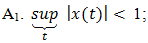 | (1a) |
 | (1b) |
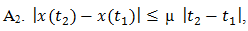
 a real positive constant and (t1, t2) any real pair.Although the Lipschitz condition (1b) implies the continuity of x(t), it does not imply either its boundedness or differentiability. Nevertheless, if the first derivative x’(t) of x(t) exists and is uniformly bounded, i.e., if
  | (1c) |
it then follows (from Rolle’s theorem) that (1b) holds with the choice 
2. The Pseudo – Static View of Natural PWM
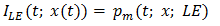
Implementation of natural PWM by the ramp-intersective method is depicted in detail in Figure 1(a). The modulation is either single-edge (SE) or double-edge (DE), depending on whether one or both edges of the pulse are allowed to shift in time. Moreover, SE decomposes into exclusively trailing-edge (TE) or exclusively leading-edge (LE).As seen from Fig. 1(b), the TE pulse train pm (t; x; TE) is generated by comparing x(t) to the ramp r(t) of slope 2/T in every interval (kT, (k+1)T). The comparator returns the value 1 if the difference x(t)-r(t) is positive and the value 0 if not. Similarly, the LE pulse train pm (t; x; LE) in Fig. 1(c) is obtained by comparing x(t) to the ramp of slope -2/T. Lastly, the DE pulse train pm (t; x; DE) in Fig. 1(d). utilizes the two dashed-line ramps rN (t) and rP (t) of slopes -4/T and 4/T to fix the location and width dk-ck of the corresponding pulse. Quantitatively, the comparator reads 1 iff x(t)-rN (t) and x(t)-rP (t) are both positive and reads 0, otherwise. | Figure 1. The Generation of Natural TE, LE and DE by ramp-intersection |
Four facts of interest emerge that are worth singling out:1. Periodicity of the ramps does not imply that of any of the three pulse trains;2. For the TE case the leading edge is fixed at kT and the trailing edge can move, for the LE case the trailing edge is fixed at (k+1)T and the leading edge can move, while in the DE case both edges can move and no symmetry about the (k+1/2)T line need exist;3. Each of the three pulse trains contributes only one pulse to every time slot 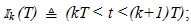 4. Examination of Fig. 1(a) reveals that the ramp of slope 2/T intersects -x(t) at the same instant that the ramp of slope -2/T intersects x(t). From this equality one easily infers the 1’s complement identity
 | (2) |
a useful algebraic result2. Any one of the pulse trains, be it TE, LE or DE, may be viewed as a pulse-coded version of an information bearing signal x(t) and knowledge of their spectral content can be essential. The pseudo-static approach to deriving this content begins by considering the TE, LE and DE trains as created in two separate steps.In the first, the trailing edge, leading edge and the two edges of 50% duty cycle periodic waveforms p(t), p(t-T/2) and p(t-T/4) of period T are shifted statically by the respective amounts τT/2, τT/2 and τT/4 in the directions indicated in Fig. 2. At this stage τ is considered to be a constant parameter subject to the sole inequality | (3) |
Pulse widening occurs if τ > 0, narrowing if τ < 0 and the numerical changes in width are less than T/2.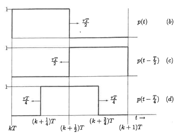 | Figure 2 |
Denote the periodic extensions of period T of these three modified pulses by  and
and  Each possesses a Fourier series expansion in t whose coefficients depend on the parameter τ. Substitution of x(t) for τ defines corresponding functions of time
  and
and  In the second step it is accepted, often on physical grounds, that the “approximations”
  | (4) |
 | (5) |
and  | (6) |
are sufficiently accurate to be of engineering significance. It perhaps is unexpected to discover that this conjecture is more than right on the mark.The Pseudo-Static (PS) Theorem: Let x(t) satisfy assumptions A1 and A2. Then | (7) |
 | (8) |
and 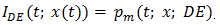 | (9) |
As an excellent illustration of the power of this theorem we shall use it to routinely derive series expansions for TE, LE, and DE natural PWM.In the interval (0, T), 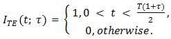 | (10) |
Hence the coefficients cr in its complex Fourier series are given by | (11) |
and 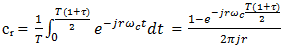 | (12) |
 | (13) |
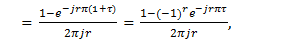
where, 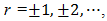 and
and  Consequently (easy details omitted),
 | (14) |
It then follows from (7) and (2) that  | (15) |
and | (16) |
As regards the DE pulse train, observe that in (0,T)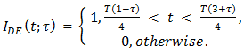 | (17) |
Therefore co = ( 1 + τ )/2 and | (18) |
where, 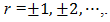 Accordingly, (some details omitted)3,
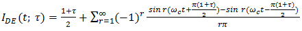 | (19) |
 | (20) |
so that | (21) |
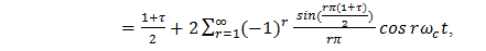
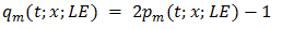
Unlike TE and LE, in DEPWM all carrier harmonics are suppressed, a possible advantage for some telecommunication applications [4].Instead of p(t), p(t-T/2) and p(t-T/4), Song and Sarwarte choose to work with the unmodulated carriers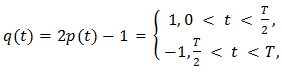 | (22) |
q(t-T/2), and q(t-T/4). Concomitantly,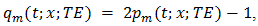 | (23) |
 | (24) |
and | (25) |
A quick check confirms that  | (26) |
 | (27) |
and | (28) |
agree with Equations (37), (44) and (63) in [2].
3. Solution of a Classical Problem
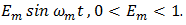
The availability of time-domain expansions for the various pulse trains almost invariably simplifies the derivation of their spectral properties.Example: Determine the spectrum of the TE pulse-train pm(t; x; TE) in (15) under single-tone modulation 
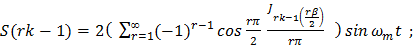
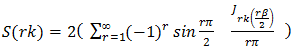
 Solution: It is first necessary to find the frequency content of the second sum S2(t) in (15). Evidently4,
  | (29) |
 | (30) |
 | (31) |
 | (32) |
 | (33) |
By extracting the n = 0 component of (32) and adding it to the sum  | (34) |
In (15) we obtain the complete decomposition | (35) |
where | (36) |
The original proof of this result by WR Bennett in 1933 was accomplished with the aid of a double Fourier series technique [7,8].
4. Proof of the PS Theorem
Consider justification of equation (9) and recall that  represents the periodic extension of the modified pulse shown in Fig. 2(d), obtained by shifting the leading and trailing edges of p(t-T/4) to the left and right, respectively, by the same amount τT/4. The resultant modified pulse has width T(1+τ)/2. Write
 | (37) |
What must be established is that  | (38) |
Let  fixed, but arbitrary, and note that
  | (39) |
Is the value of  | (40) |
for t = t0. Since f(t) is a period T periodic function, its structure is known. Indeed, in  is a unit-magnitude rectangular pulse with leading and trailing edges located at the respective translates
 | (41) |
of the points T(1 - x(t0))/4 and T(3 + x(t0))/4 on the t-axis of I0 (T) = (0 < t < T). Accordingly, f(t0) = 1, iff  | (42) |
and equals 0 otherwise. Equivalently, such is true iff | (43) |
Or, expressed more compactly, iff x(t0) > rp(t0) and x(t0) > rN(t0), where  | (44) |
are the equations in  of the positive and negative slope dashed-line ramps shown in Fig. 1(a). To sum up, for-t in
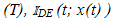 = 1 iff x(t) is greater than both rp(t) and rN(t) and is 0 if not, precisely the rule prescribed in section 2 for the ramp-intersective formation of the pulse train pm(t; x; DE) in Fig. 1(d). The proofs of (7) and (8) proceed along very similar lines5. Hence, guided by footnote 5 we obtain, without difficulty,
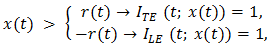 | (45) |
where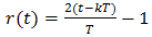 | (46) |
is the equation in  of the positive-slope solid-line ramp shown in Fig. 1(a). Moreover, if > in (45) is changed to <, 1 is changed to 0, Q.E.D.
5. Overview
The pulse trains in Figs. 1(a), (b), and (c) are monopulse, in the sense that each contributes only a single pulse to every interval  This need not be true in general, but is always achievable by making T sufficiently small, i.e., by choosing the sampling rate 1/T large enough. For the proof, assume that x(t) makes contact with the ramp r(t) in (46) at distinct points t1, t2, in
  Then x(t1) = r(t1), x(t2) = r(t2) and
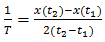 | (47) |
follows. Consequently, in view of assumption A2,  | (48) |
Clearly, when 1/T > µ/2, (48) is contradictory and distinct multiple ramp contacts are precluded.6 But a pulse train generated without multiple ramp contacts is necessarily mono.If the convergence of the several infinite series is accepted [7], it appears that our proof of the PS theorem is of a truly elementary character. It relies almost entirely on the realization that the value of  for any given t=t0 equals the value of f(t) =
  for t=t0. Since f(t) is of period T and of known rectangular shape fully defined by p(t) and x(t0), this value is immediately determined.Also, as a matter of practical concern, it is useful to know that bandlimited functions x(t) of finite energy are automatically bounded and always satisfy assumption A2 [9]. In this case it is possible to enforce A1 by ordinary amplitude scaling.
6. Demodulation of Single-Tone Modulated TE, LE and DE Pulse Trains
The Bennett decomposition of the TE pulse train pm(t; x; TE) generated by single-tone modulation 
 is displayed in equations (35) and (36). Close examination under the assumption
  reveals that ideal low-pass filtering of radian bandwidth
  will, when applied to pm(t; x; TE) as input, produce an output which in addition to the information bearing waveform (1+x(t))/2, contains other terms that account for distortion and are contributed by the double sum
 | (49) |
Introduce the positive parameter  Then k is > 1 and
  | (50) |
Consequently, a component (50) in (49) lies in the passband of the filter (and therefore adds to the distortion), iff  or, iff the integers r and n obey the inequality
  | (51) |
i.e., iff | (52) |
Let  and
and  denote, respectively, the largest integer
  and the smallest integer
  From (52)7
 | (53) |
Evidently, if  is an integer,
  and the allowed values of n are given by
  | (54) |
But if  is not an integer,
  and now only pairs
 | (55) |
are permitted. Correspondingly, if k > 1 is prescribed in advance and  denotes the distortion produced by term r in (49), then for rk an integer,
  | (56) |
When, however,  is not an integer, it may be rewritten as
  where
where  so that
  | (57) |
is a weighted sum of two complementary subharmonics of  8 Of course, as is obvious,
  an integer implies all
  integers, whereas
  not an integer implies that some
  are not integers. In the first case the total distortion is of the form
  where
where  is the sum over
  of the coefficients of
  in (56), while in the second the sum of the
  in (57) always includes subharmonics. In fact, with irrational
  all distortion is subharmonic.9It should now be apparent that the normalized quantity
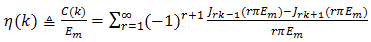 | (58) |
is an appropriate measure of total distortion when  is an integer greater than one.10 Some simplification is possible, for replacement of
  and
and  in the Bessel function identity [11]
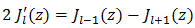 | (59) |
transforms (58) into 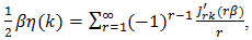 | (60) |
a series of the Kaptyen type [11], in which the modulation index  because the modulation depth
  satisfies
  Let
Let  and suppose that
  For fixed
  and
and  is positive and decreases monotonically as
  .11Proof. According to Watson [11, Pgs. 253,254] for
  and
and  both
both  and
and  when viewed as functions of
  with
with  held fast, are positive and decrease monotonically as
  increases. To make use of the second of these two properties, write
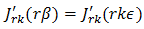 | (61) |
and observe that an increase of  may be interpreted as an increase of
  from
from  in the function
  without change in
  Q.E.D.Corollary (important): For,
  the quantities
  in (60) are positive and decrease, monotonically, to zero as
  Thus (60) is an alternating series that meets the Leibnitz null-monotone requirement. It therefore converges [12] and the remainder
  after
after  terms is always numerically less than the numerical value of the first term neglected, i.e.,
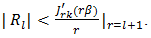 | (62) |
It seems evident from symmetry considerations that equation (60) for  should also be valid for single-tone modulated LE pulse trains. A more informative analytic proof, however, is had by referring back to (35) and (36) to conclude with the help of the 1’s complement identity (2), that all LE distortion is contributed by the terms in the sine-wave summation12
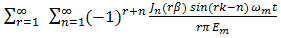 | (63) |
that get passed by the low-pass filter. Accordingly, addition of the particular terms corresponding to  and
and  etc. leads to (58) and then quickly to (60), provided
  is an even positive integer.13 Of course
  and
and 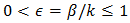 are again necessary constraints. To demonstrate the applicability of (60) to single-tone modulated DE pulse trains, we set
  in (21) and then perform spectral analysis in the manner used to derive the Bennett partition in equations (35), (36). As a first step we ask the reader to verify that the second term in (21) may be rewritten in the expanded form
 | (64) |
With the aid of the identity  we readily see14 that the only sine waves that can contribute to distortion are those of radian frequencies
  contained in the sum
  | (65) |
Assume, once again, that  is an even integer
  and let us compute
  for the three permitted values
 | (66) |
 | (67) |
and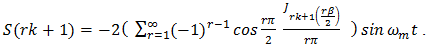 | (68) |
Since  is an irrelevant and removable DC pedestal, the sum of the coefficients of
  in (66) and (68), divided by
  is the obviously correct measure of total normalized distortion
  Hence
Hence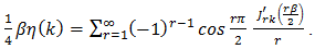 | (69) |
But  for r odd and equals
  for
for  even. Concomitantly,
 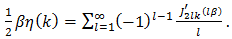 | (70) |
This is an alternating series of the Leibnitz null-monotone type when  in addition to being an even integer
  also meets the requirement
  15Demodulation Theorem: The total distortion
  incurred by using ideal low-pass filtering to demodulate the three pulse trains created by natural single-tone pulse-width modulation is determined from equations (60) and (70). Specifically, assume
  to be an integer
  Then 1. for TE use (60) with
  2. for LE use (60) with
  3. for DE use (70) with
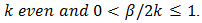
7. Numerical Results for the Design Engineer
Problem Statement for the EngineerThe problem statement of interest to the design engineer begins with reference to footnote 10, equation (59b), of this paper. There,  is seen to quantify the level of distortion to be tolerated in the process of demodulation of x(t). Equation (60) shows that
  is calculated from a series whose terms are composed of Bessel function derivatives. Furthermore, (60) also reveals that
  is a function of k and β. So, the task for the engineer is to determine the smallest k for a given β and a given upper bound on
  Equation (60) applies in the cases of TE and LE PWM, while (70) applies to the case of DE PWM. Initially, the discussion will center on (60) with the understanding that (70) is understood similarly and is appropriately clarified in the sequel. Computation of Bessel Function Series CoefficientsNumerical tabulation of the series coefficients makes use of (59) combined with the Bessel function tables found in [13]. The coefficient data is tabulated and appears in Tab.’s 1(a) and 2(a). We will need to use this data both to estimate
  and to estimate the percent error associated with our estimate of
  Theoretical underpinnings are developed next to make effective use of this numerical data to solve the design problem as stated.Theoretical Underpinnings for Numerical ProceduresAbsent a closed form solution for the value of
  in (60), one may then proceed to numerically estimate
  We are fortunate that this series is a member of the class of alternating series known as the Leibnitz null-monotone class. This is the best of all series with many desirable properties, convergence among them, that permit numerical estimation of
  We begin by writing
  as follows. Let
 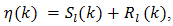 | (71) |
where  represents a finite sum obtained by taking the first l terms in (60) and the infinite series
  is the remainder. We will represent the approximation of
 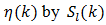 as
as 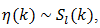 | (72) |
when l is to be large enough to result in a satisfactory estimate. The formal solution to this estimation problem [15] can be stated as 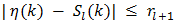 | (73) |
where,  is used designate the real number which is the absolute value of the first term of
  in (71).While (73) provides an answer to the number of decimal places of agreement one can expect in (72), an additional figure of merit which permits us to estimate the “percent error” associated with our estimate of
  is useful. This “percent error” is designated as
  and is formulated16 as
 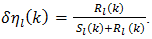 | (74) |
An admissible17  as well as it’s associated
  must converge to a nonzero17 value. Rewriting (74) by dividing by
  is then well-defined for any l, infinity included. If we also make use of the triangle inequality we can write an upper bound for
  as
as 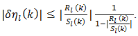 | (75) |
The properties of alternating series alone [15] permit us to bound  in (75) by
  and write
 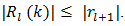 | (76) |
Combining (75) with (76) we recognize that in place of a specific series like (60), we have focused our considerations on the properties of an entire admissible class of alternating series. We have then proven the following Theorem: The percent error  is bounded by (77) when partial sums
  of an admissible alternating series
  are employed in its approximation. Thus,
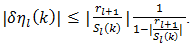 | (77) |
Observing the null-monotone property of such series, we are permitted to state that18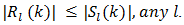 | (78) |
This result calls attention to the fact that as l increases the quantity in (79) holds for any admissible  namely,
 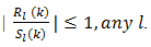 | (79) |
As l increases the left side of (79) becomes ever smaller18 than the numerical bound of 1 located on the right side of (79). When l is sufficiently large to satisfy (73), (77) may then be simplified using [16, # 748, p. 88]. Upon replacing  by
by  we have proven the following Corollary: For l large enough (80) suffices as an upper bound19 to the percent error for the admissible class of alternating series. Thus,
 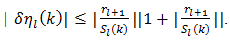 | (80) |
Lastly, although  is explicitly unknown, we can bound its values above and below with the partial sums
  For l odd it is clear [17, p. 371] that the following is true,
 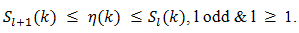 | (81) |
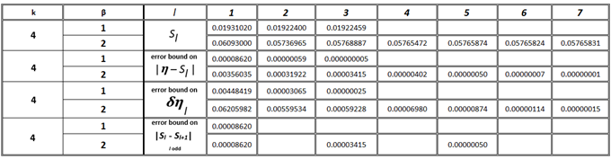
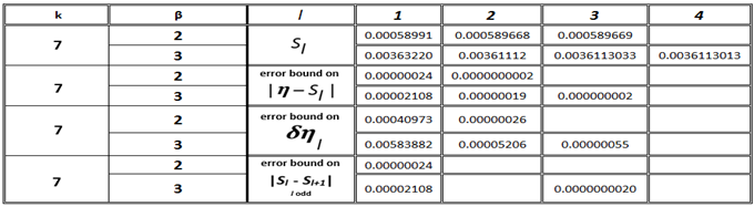
This property provides numerical results which complement (77). Equations (71) to (81) will be applied to the Bessel function series coefficients located in Tables 1(a) and 2(a). These tables are structured in the following way; the rth row along any column represents the value of the rth term in (60) excluding the  factor. Each column represents a given choice of the variables β and k. In each column as terms decrease monotonically the value of the term is taken as zero when at least 7 of the first digits are zero. Partial sums
  and bounds on the error
  for various choices of the integer l are displayed in Tab.’s 1(b) and 2(b) for selected values of k and β.
 Table 1(a). Bessel Function Derivative Coefficients
 |
| |
|
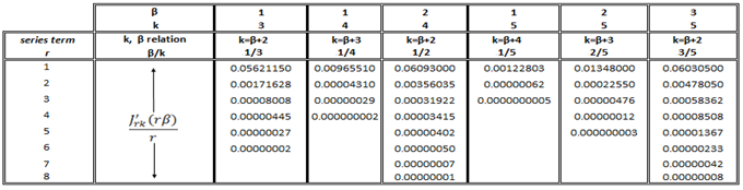
Table 1(b). Estimation of η by Sl using coefficients from Table 1(a)
 |
| |
|
Table 2(a). Bessel Function Derivative Coefficients
 |
| |
|
Table 2(b). Estimation of η by Sl using coefficients from Table 1(a)
 |
| |
|
The information in Tab.’s 1(b) and 2(b) permits us to calculate  from its corresponding estimate
  To do this simply multiply the appropriate
  by “2” (i.e.; see “2” in footnote 10, (59b)). Further multiplication of
  by “100” calculates the percent error in the demodulation of x(t). Information gathered in this way was used to construct a design graph for TE and LE PWM in Fig. 3. Fig. 3 displays percent distortion error vs β for various k values. Thus, the engineer may readily choose the smallest sampling rate k consistent with performance requirements for such links. An entirely analogous development applies to equation (70) for DE PWM whose results appear in Fig. 4.
 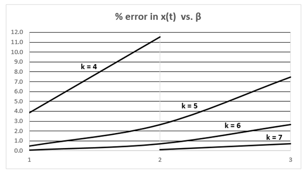 | Figure 3. Summary of distortion vs. β & k from equation (60) for TE & LE |
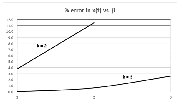 | Figure 4. Summary of distortion vs. β & k from equation (70) for DE |
8. Application of the Demodulation Theorem
An application of the demodulation theorem is in order and demonstrates the utility of the results of the previous section. Application Example: Consider TEPWM and determine the sampling rate k required for β = 2 in order to achieve at most 3% total harmonic distortion. Explore similar design choices for LEPWM and DEPWM.Solution: For TEPWM the requirements stated in part 1 of the demodulation theorem for (60) allow for an otherwise unrestricted choice of k. The results contained in Fig. 3 suggest that an appropriate choice for k is k = 5. For LEPWM the requirements of part 2 of the theorem require the additional constraint that k be an even number if (60) is to describe the distortion. Again, referring to Fig. 3 we see that k = 6 suffices in order to meet (and in fact exceed) the required distortion level. For DEPWM the requirements of part 3 of the theorem suggest that upon replacing (60) by (70) and referring, now, to Fig. 4 the choice of k = 3 exceeds the requirements and is smaller than the value of k for the TE and the LE cases just considered. So, an added bonus is achieved with DE since we only require half of the k! Thus, DE is superior to TE and LE. Physically, DE uses double the number of samples per interval explaining why only half the k is required.
9. Comparison with the Work of Others
Holmes, et. al., [10], use a double Fourier series method to develop a time domain equation (p. 111, eq. 3.26) for the modulated signal which is similar to either (15), (16), or (21) as developed in the present work using the pseudo-static methodology. Distortion is defined differently for their application. Higher k values were required to lessen the effects of distortion as compared to the work described herein. This exhibits a certain consistency with the present work; Holmes work, however, is otherwise very distinct from the present work. The work summarized in Wilson, et. al. [14] provides a more interesting comparison as there is greater overlap in the work. Equation 4.1 in chapter 4.0, [p. 96, 14] is also similar to (15), (16), or (21) in the present. Wilson, et. al. use Equation 4.8, [p. 112, 14] is to estimate distortion error. Equation 4.8 [p. 112, 14] is a truncated version of equation 4.1, [p.96, 14]. This is similar in manner to the way the present authors have analyzed the distortion error with the exception that l is limited to 1 in [14]. The contrast between the procedure used by Wilson, et. al., [14] and the present authors is that the present authors have the benefit of knowing that (60) is an alternating series with many properties. It seems logical to assume that absent this information, Wilson, et. al. would likely do the next best thing which is to engage in experimentation to lend independent validity to their process of truncation. This is illustrated in results displayed in Fig. 4.15 [p. 112,14]. The work of Wilson, et. al. and the present work are somewhat complementary in this regard.
10. Conclusions
A proof is provided herein for the Pseudo-Static theorem. This proof is elementary in nature. The Pseudo-Static theorem establishes the exactness of Pseudo-Static spectral analysis, without the need to introduce superfluous constraints. This is physically significant and is in complete agreement with the work of Bennett, op. cit.. The distortion is understood for three types of natural PWM and is quantified in terms of a pair of alternating series each of which exhibits the Leibnitz null-monotone property. The benefit of such series is used to great advantage in numerical work, especially when presented in a tabular and graphical form which permits the design engineer to easily understand the distortion in terms of the parameters β and k.
Notes
1. Natural PWM is accomplished by means of the ramp-intersective method described in section 2.2. 1), 2), and 4) require little explanation and 3) holds whenever 1/T > µ/2 (Proof postponed).3.  4.
4.  is the Bessel function of the first kind of order n and argument z [3]
 and Im[z] is the imaginary part of the complex number z.5. For example, in Ik (T) the function f(t) = ILE (t; x(t0)) is a unit-magnitude rectangular pulse with leading and trailing edges located at T(1-x(t0))/2+kT and (k+1)T, respectively. Hence f(t0)=1 iff t0 > T(1-x(t0))/2+kT, i.e., if f x(to) > 1-(t0-kt)2/T =-r(t0), etc..6. Naturally, 1/T > µ/21/T > µ/4 and distinct multiple contacts with the ramps rp(t) and rN(t) in (44) are similarly ruled out.7.
  and
and  8. Specifically,
  9. These subharmonics are often partly responsible for unacceptable pulse-train jitter at the receiving end of a fiber-optic data link [10]10. With this notation the filter output may be expressed as
  | (59a) |
Clearly, the use of the estimator  | (59b) |
for  entails a
  percent error in the estimate of either
  11.
11.  12.
12.  13.
13.  when the integer
  is even because
  and
and  14. The n = 0 term lies outside the filter bandwidth and may be ignored.15.
  is an instance of
  with
with  and
and  16. The actual percent error is of course obtained after multiplication of
  obtained in (74) by 100.17. We of course assume that
  for the alternating series are each nonzero and of like sign. A series constrained in this manner necessarily converges to a finite nonzero sum. If such were not true in PWM, say, there would be no distortion error to consider in x(t) to begin with. 18. It is clear [15] that
  In general [15]
  where L is a finite limit. It should be clear that in the context of this paper L is required to be nonzero for admissibility.19. No claim is made as to the optimality or uniqueness of this bound compared to other bounds used herein or elsewhere.
References
| [1] | Starr, A.T., 1952, Radio and Radar Techniques, Pittman and Sons, LTD (London). |
| [2] | Zukui Song, Dilip V. Sarwate, The Frequency Spectrum of pulse width modulated signals, 20003 Elsevier, Signal Processing, vol 83, pgs. 2227-2258. |
| [3] | E.T. Whittaker, G.N. Watson, A course of Modern Analysis, p. 132, 4th edition, Cambridge 1952. |
| [4] | Suh, S.Y., Pulse Width Modulation for Analog Fiber-Optic Communication, Journal 0f Lightwave Technology, Vol. LT. 5, No. 1, January 1987. |
| [5] | Z. Ghassemlooy, B. Wilson, Optical PWM Data Link for High Quality Video and Audio Signals, IEEE Transactions on Consumer Electronics, vol. 40, No. 1, February 1994. |
| [6] | B. Wilson, Z. Ghassemlooy, Pulse time Modulation techniques for optical communications: a review, IEE Proceedings J, Vol. 40 No. 6 December 1993. |
| [7] | W. R Bennett, New Results in the Calculation of modulation components, Bell Syst. Tech, J, 1933, 12,pp. 228-243. |
| [8] | H. S. Black, Modulation Theory, Van Nostrand, New York, 1953, Chapter. |
| [9] | A. Papoulis, Signal Analysis, McGraw-Hill, New York, 1977, pp. 196,197. |
| [10] | D. Grahme Holmes, Thomas A. Lipo, Pulse Width Modulation for Power Converters, IEEE Press, Wiley Interscience, 2003. |
| [11] | G. N. Watson, A Treatise on the Theory of Bessel Functions, Cambridge University Press, Second edition, 1966. |
| [12] | T. J. Bromwich, Theory of Infinite Series, McMillian and Co., Limited, Second Edition, 1949. |
| [13] | E. Jahnke and F. Emde, Tables of functions With Formulae and Curves, Dover Publications, New York, pp. 170-182. |
| [14] | B. Wilson, Z. Ghassemlooy and I. Darwazeh, “Analogue Optical Fibre Communciations”, IEE Telecommunications Series 32, 1995. |
| [15] | K. Knopp, “Theory and Application of Infinite Series”, Blackie & Son, 1944. |
| [16] | B. O. Peirce, “A Short Table of Integrals”, Ginn and Co., 1929. |
| [17] | R. Courant, “Differential and Integral Calculus”, Vol I, Interscience, 1937. |

 Abstract
 Reference
 Full-Text PDF
 Full-text HTML