-
Paper Information
- Paper Submission
-
Journal Information
- About This Journal
- Editorial Board
- Current Issue
- Archive
- Author Guidelines
- Contact Us
American Journal of Signal Processing
p-ISSN: 2165-9354 e-ISSN: 2165-9362
2018; 8(1): 9-19
doi:10.5923/j.ajsp.20180801.02

Optimization of Transformation Matrix for 3D Cloud Mapping Using Sensor Fusion
 Abstract
 Reference
 Full-Text PDF
 Full-text HTML
Hai T. Nguyen, Viet B. Ngo, Hai T. Quach
Department of Industrial Electronic-Biomedical Engineering, Faculty of Electrical-Electronics Engineering, HCMC University of Technology and Education, Vietnam
Correspondence to: Hai T. Nguyen, Department of Industrial Electronic-Biomedical Engineering, Faculty of Electrical-Electronics Engineering, HCMC University of Technology and Education, Vietnam.
| Email: |  |
Copyright © 2018 Scientific & Academic Publishing. All Rights Reserved.
This work is licensed under the Creative Commons Attribution International License (CC BY).
http://creativecommons.org/licenses/by/4.0/

This paper proposes an optimization method of transformation matrix for 3D cloud mapping for indoor mobile platform localization using fusion of a Kinect camera system and encoder sensors. In this research, RGB and depth images obtained from the Kinect system and encoder data are calculated to produce transformation matrices. A Kalman filter algorithm is applied to optimize these matrices and then produce a transformation matrix which minimizes cumulative error for building 3D cloud mapping. For mobile platform localization in an indoor environment, a SIFT algorithm is employed for feature detector and descriptor to determine similar points of two consecutive image frames for RGB-D transformation matrix. In addition, another transformation matrix is reconstructed from encoder data and it is combined with the RGB-D transformation matrix to produce the optimized transformation matrix using Kalman filter. This matrix allows to minimize cumulative error in building 3D point cloud image for robotic localization. Experimental results with mobile platform in door environment will show to illustrate the effectiveness of the proposed method.
Keywords: Kinect camera, Transformation matrix, SIFT algorithm, Kalman filter, 3D point clouds, Encoder data
Cite this paper: Hai T. Nguyen, Viet B. Ngo, Hai T. Quach, Optimization of Transformation Matrix for 3D Cloud Mapping Using Sensor Fusion, American Journal of Signal Processing, Vol. 8 No. 1, 2018, pp. 9-19. doi: 10.5923/j.ajsp.20180801.02.
Article Outline
1. Introduction
- An automatic mobile platform designed to automatically move based on 3D mapping has attracted researchers in recent years. In particular, robotic mapping is one of the most vital tasks in automatic robotic applications, in which the robot has to be supported the model of the navigational space in order to locate itself when moving. Thus, the map is essential for path planning processes in proposing the roadmap to target positions [1].The robotic mapping is divided into 2D and 3D mappings. The 2D mapping has some disadvantages compared with 3D mapping. It means that the applications using sonar or laser sensors in navigation with 2D mapping has its drawbacks [2-4]. One of the great drawbacks of using the 2D mapping for accurate robotic locations is the lack of information in the third space dimension [5]. For improving the negative trends of 2D planning methods, the 3D mapping algorithms have been continuously developing with the supports of famous classical findings. Therefore, a Simultaneous Localization and Mapping (SLAM) algorithm is applied with 3D mapping methods for determination of the 3D model of large scale environments [6, 7]. The result is that the 3D mapping methods have effectively employed for building robotic mapping.The quality of 2D mapping with obstacles from surroundings using sonar or laser sensors [8] is mainly determined due to its limitations. In particular, the sonar sensors used to obtain the ranges from the robot to surrounding obstacles just show obstacle information on the beam plane where the sensors are installed. For improvement of using the sonar sensor, the stereo camera system were used to take advantage of building 3D mapping with obstacles [8-11], but the calculation time to reconstruct the 3D ranging information from stereo images is expensive and it price is problem.The Kinect RGB-D sensor (Kinect camera system) has been used to replace the stereo camera system for robotic localization [12]. This kind of the RGB-D sensor has not only the suitable accuracy, but also allow to calculate processing time with the fast speed. In addition, it is much cheaper than the 3D sensor with the same functions and easy to install for use. Therefore, algorithms have been applied using RGB-D sensors for determining the moving space as well as identification and positioning in the space of self-propelled robots in recent years [13-15]. One disadvantage of this RGB-D sensor is that its depth information is often noisy. Therefore, if a robot equipped with the Kinect moves long distances, the accumulated error for robotic localization gets over time [16]. There have been many proposed methods such as considering noise characteristics, dependently updating distances to reduce this error as well as to improve the accuracy of 3D mapping [17-19]. In addition, for determination of feature-based image, the method of the feature-based image registration includes two parts: interest point detection and interest point description. Moreover, this method is based on the basis of Scale-Invariant Feature Transform (SIFT) algorithm for noisy reduction [20-22]. The features extracted also have scale and rotation-invariant performance with respect to illumination change, affine and perspective transformation. In addition to three aspects of repeatability, distinctiveness, and robustness, computation cost is not expensive.The Kalman filter has many uses in applications of control, computer vision, filter and navigation [23-24]. In particular, the Kalman filter has been applied to track a vision object, in which it can be used to predict a process state. In addition, the Kalman filter was used in reconstructing medical images for contrast and transparency. In the robotic localization, the Kalman filter is employed to optimize the robotic position by processing the transformation matrices built from data obtained the Kinect camera system and the encoders.In this paper, an optimization method by processing the transformation matrices built from sensor data for accurately reconstructing the 3D mapping. A Kinect (RGB-D) camera system is installed with the robot’s cage to continuously capture the separate 2D image frames and 3D point clouds. All corresponding 2D points between the two consecutive image frames are estimated using the SIFT algorithm to produce the first transformation matrix. While the encoders equipped with the robotic wheels for calculating the second transformation matrix. The Kalman filter is applied to optimize them and create the most accurate transformation matrix. The next section of the paper presents in more details with the effectiveness of experimental illustrations.
2. Description of Mobile Platform
- In this research, the hardware system architecture of the mobile platform (robot) includes a Kinect RGB-D sensor V2 connected to a personal computer (PC) and other devices for processing data and controlling the robot. After navigation tasks for control of the differential robot, the velocity signals from the PC through Driver controller are sent to the left and right wheels. In addition, two encoders are installed with motors to send distance signals to the PC through Driver controller as shown in Figure 1. Finally, all mappings and localization processes are displayed on the LCD monitor during movement of the robot.
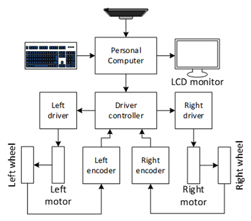 | Figure 1. Block diagram of the hardware system of the mobile platform |
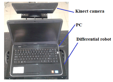 | Figure 2. Robot model with the Kinect RGB-D sensor V2 and PC |
3. Methods for Localizing and Mapping
- The description of 3D mapping and methods for calculation of robotic localization are represented in the paper. The 3D mapping procedure shows conversion of 2D image into 3D image and solutions for image matching, synthesis, concatenation to create the optimized transformation matrix.
3.1. SIFT Algorithm for Detector and Descriptor of Features
- For calculation of image features, the SIFT algorithm for feature detector and feature descriptor is employed [22]. The SIFT algorithm allows to detect features of 2D and 3D images, including two main steps: the first step is the feature detection and the second step is the feature description. In practice, the locations of stable features are detected, and then each feature is described so that it can be stable in various scale and direction appeared in the detecting images. Each keypoint when finishing description has the description of multiple direction vectors as shown in Figure 3.
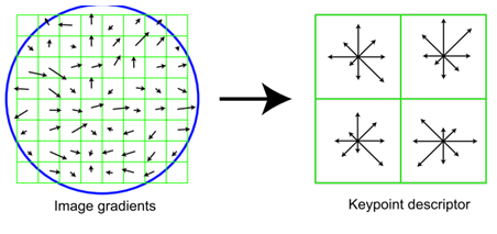 | Figure 3. Image gradients and keypoint descriptor |
 is satisfied and its equation is described as follows:
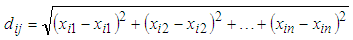 | (1) |
3.2. Calculation of Transformation Matrix
- For reduction of cumulative errors, transformation matrices built from data of the Kinect camera and encoders are considered. 2D images are calculated to convert into 3D images to create the matrices.
3.2.1. Conversion of 2D Image into 3D Image
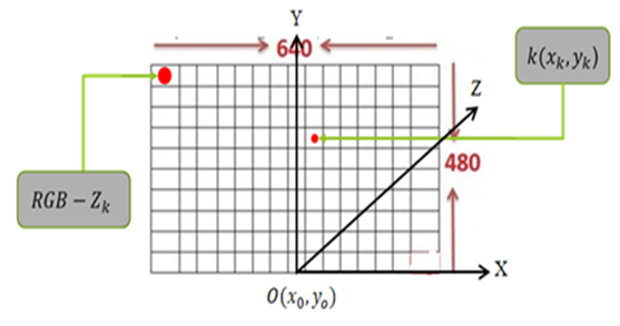
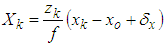
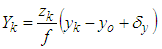
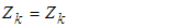
- A Kinect camera system with a main structure, consisting of a color camera, gives a 2D color image of 640x480 pixels. Each pixel will contain 3 RGB colors. In addition to the Kinect camera, the infrared light allows to captures the depth from the camera to the image plane as shown in Figure 4. Therefore, with many depth distances in the image, one can obtain the set of depths.
 | Figure 4. Description of the 3D image |
 | (2) |
 | (3) |
 | (4) |
3.2.2. SIFT Algorithm for Determination of Image Feature
- After analyzing the features on two 2D images, a set of vectors describing the characteristics of the two 2D images are obtained. Therefore, the set of the first vectors with the features is compared to that of the second vectors for determining similar points. If the number of matching points satisfies the requirement, it means that two 2D images are similar (considered as one object captured at two different angles).Thus, the process of finding pairs of similar features is carried out in three steps: finding the location of the feature point on two 2D images; describing the characteristics of each location found using the SIFT algorithm; and identifying pairs of similarities on the two images captured by the camera. After finding the similar point pairs in the two 2D images, one can determine the coordinates of the similar pairs in the two corresponding 3D clouds of the two 2D images.From the coordinates of the similar points in the two 2D images, one can derive the coordinates of the corresponding point pairs on the 3D cloud based on (2), (3) and (4). In particular, the first 2D image gives a 3D cloud corresponding to the 3D coordinate (O0X0Y0Z0) and The second one has the corresponding coordinate (O1X1Y1Z1). Thus, after identifying the similar points with the 3D coordinates between the two 3D clouds, it can be paired these similar points.
3.2.3. Synthesis of Two 3D Point Clouds
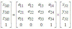
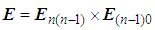
- Assume that there are two sets of 3D points which are P0 with the coordinate (O0X0Y0Z0) and P1 with the coordinate (O1X1Y1Z1) acquired from the RGB-D camera. Moreover, the rotation and translation matrix E is described as follows:
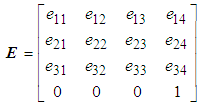 | (5) |
 | (6) |
 | (7) |
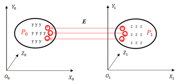 | Figure 5. P1 and P0 are the transformation matrices |
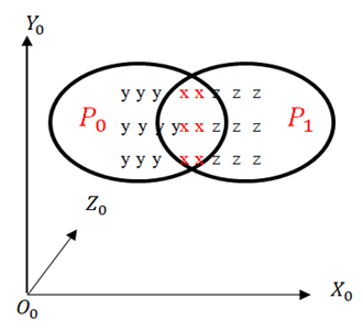 | Figure 6. Two clouds have the similar point pairs x with red color |
3.2.4. 3D Point Cloud Concatenation
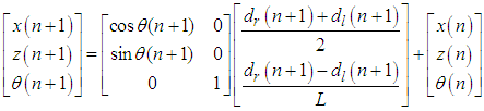
- All 3D point clouds are concatenated together based on the pair of the transformation matrices. Thus, for (n+1) clouds, the transformation matrix is calculated by the following formula:
 | (8) |
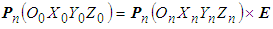 | (9) |
3.2.5. Determination of the Transformation Matrix from Encoder Data
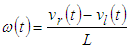
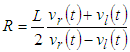
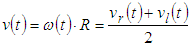
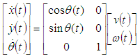
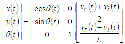
- The dynamic equation for the robot describes the relationship between the coordinates O(x,y) in the Descartes coordinate of the robot and the velocity of two robotic wheels. Figure 7 gives the model of a robot, in which the robot model will move and navigate by two wheels equipped with two encoders.
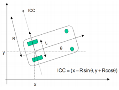 | Figure 7. Model of the mobile platform |
 | (10) |
 | (11) |
 | (12) |
 | (13) |
 | (14) |
 | (15) |
 | (16) |
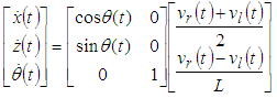 | (17) |
 | (18) |
 | (19) |
3.3. Optimization of Transformation Matrix Using Kalman Filter
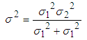
- In this project, the Kalman filter is applied to optimize the robot localization for optimizing the transformation matrix of two 3D clouds. This robot has two sets of sensors, in which the first sensor is a Kinect camera system that collects RGB data images with depth and the second one has two encoders installed with wheels for collecting data of the rotation wheels.Assume that the Kinect data provide the estimated position 𝑞1 of the robot at time t, data of the encoders show the estimated position 𝑞2 of the robot at time (t + 1). These data exist Gaussian noises, called the combinational variances σ12 and σ22. A least squares technique is applied to estimate the robot position, where
 is the best estimated position of the robot and 𝑤𝑖 is the weight of the ith measurement, the estimated equation is described as follows:
 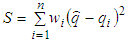 | (20) |
 equals to 0 and its equation is calculated as follows:
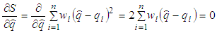 | (21) |
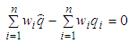 | (22) |
 | (23) |
 | (24) |
 | (25) |
 | (26) |
 | (27) |
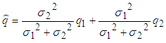
 is determined from two positions of two sets of the sensors.From Eq. (25), the best localization equation is represented as follows:
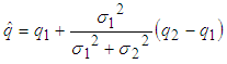 | (28) |
 | (29) |
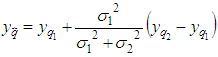
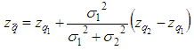
 is the most accurate coordinate of the robot and
 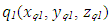 is the estimation parameter obtained from the transformation matrix E,
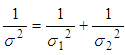
 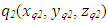 is the estimation obtained from the encoder, σ12 and σ22 are the variances representing the Gaussian signals for two positions 𝑞1 and 𝑞2. Thus, equations are determined as follows:
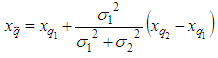 | (30) |
 | (31) |
 | (32) |
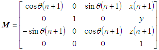
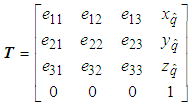
3.4. Point Cloud Transformation
- The transformation method in 3D spaces is mainly used in this project due to its suitableness and effectiveness for the transformation of the 3D point cloud. In practice, a set of 3D point cloud is transformed to other positions in the same coordinate and its equation of a single 3D point is represented as follows:
 | (33) |
 is the input point cloud,
  is the ouput point cloud and T is the transformation matrix obtained from Eq. (29).
4. Results and Discussion
4.1. Image and Point Cloud Acquisition
- The Kinect camera sensor (RGB-D camera) used in the paper produces image data comprising of RGB images with depth. Moreover, the depth image data is often pre-processed by the Kinect hardware as shown in Figure 8. In two consecutive images captured from the Kinect, point clouds contain both new and old information; consequently, the combination of them is expected to cover more additional data. The next step of concatenating process is to estimate the pixel locations of key points from the two images. Figure 9 shows two 3D clouds of one image frame at the room angle processed based on the RGB image data and depth information.
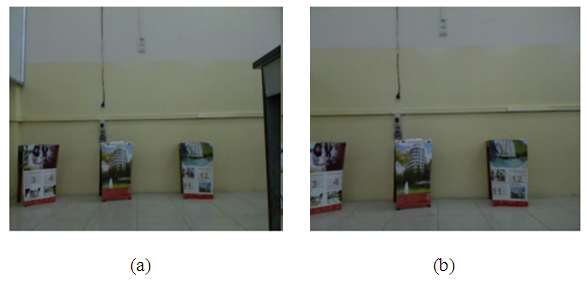 | Figure 8. Two consecutive RGB images captured from the Kinect sensor |
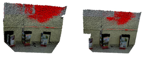 | Figure 9. 3D cloud images combined by RGB and depth images of the room space |
4.2. Key Point Estimation
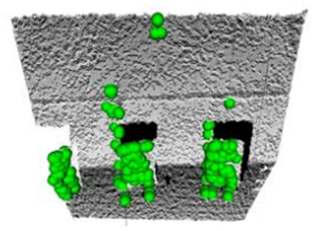
- The SIFT algorithm was applied to locate the key points in the first and second images and their characteristics are independent from scales and rotations. Figure 10 shows the key points marked in the white points. The key points are mainly focused on the areas where the difference is in high gray level. Next, each detected key point is described by a 128-dimensions vector to be able to recognize easily by using Euclid’s distance Eq. (1). The two key points are considered to be matched if the distance between their vectors is less than a pre-defined constant.
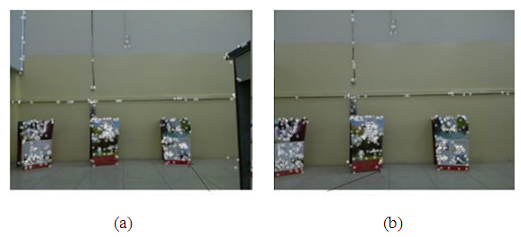 | Figure 10. Feature points of the first and second RGB images |
4.3. 3D Key Point Matching
- After estimated and described by using the SIFT algorithm, the key points on the second image are matched to their corresponding points and Figure 11 shows all corresponding key points on the first and second images. In this figure, each matching is presented by a green line connected between two key points.
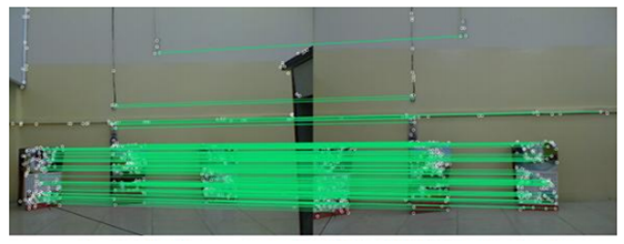 | Figure 11. Pairs of similar points of two consecutive RGB images connected in green color |
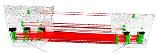 | Figure 12. Matching keypoints between the first and second 3D point clouds |
4.4. Pair Concatenation
- In Eq. (5), the transformation matrix has the size of (4×4), in which 12 parameters are unknown. Therefore, it has at least 12 pairs of corresponding points in the 3D cloud in order to infer the correct values. However, the number of corresponding points is often more than 12 due to the errors can happen when matching between two point clouds. After the transformation matrix is determined, the matrix is applied to calculate for the second point cloud in order to have the same coordinate system as the first point cloud. The experimental result of the concatenating point cloud is described in the Figure 13.
 | Figure 13. The concatenated point cloud |
4.5. Optimization of 3D Mapping Using Kalman Filter
4.5.1. 3D Clouds with Less Similar Points in the Transformation Matrix
- Figure 14 is a 3D map of the robotic path in the room environment without the Kalman filter. It is obvious that the rotating robot parts of the map occur during the grafting process, in which the right wall was broken and the left part of the room was misplaced. The cause of this error is that the number of similar points of two consecutive clouds at the location of the error is not sufficient to compute the transformation matrix. Therefore, the value of the matrix element is defined as zero corresponding to pairs of two clouds not being close together. The error value of this transformation matrix will affect all other transformation matrices in calculating.
 | Figure 14. 3D mapping with the robot path when moving around the room without Kalman filter |
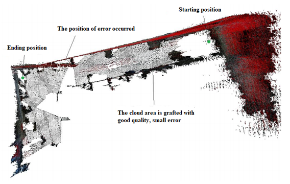 | Figure 15. 3D map of a part of the room is faulty due to cumulative error |
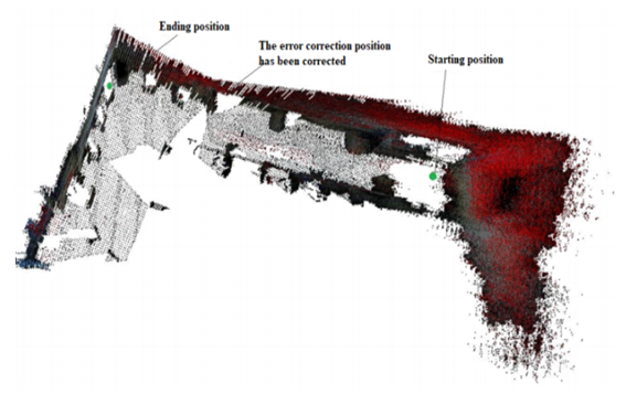 | Figure 16. 3D map of a part of the room after eliminating the cumulative error with Kalman filter |
4.5.2. Improvement of the Cumulative Error for Calculating the Transformation Matrix
- In addition, the Kalman filter improves the cumulative error in the transformation matrix calculation. Figure 17 shows the X coordinate of the robot moving a straight distance of 30cm toward the front of the Kinect camera. With 21 RGB images and depth images, we can identify 21 different coordinates of the robot to different positions. The brown line is the standard coordinates of the robot when traveling in a straight line defined in advance. When the robot moves straight in front of the Kinect camera in the direction of the Z axis, its X coordinate is zero at all positions. The green line is the value of the X coordinate of the robot measured from the encoders and it is calculated from the coordinates of the similar points. It means that the blue line tends to be far from the brown line due to the cumulative error. While the purple line determined using the Kalman filter is optimized more than the blue and green lines, so it is closer to the brown line. The demonstration result of the robot position error shows that it has been minimized using the Kalman filter and the encoder signals.In similarity, the graphs with the Y coordinates of the robots at other positions were calculated, in which the blue line is determined the coordinate from the similar points, the green line is calculated based on the encoder signals and the purple one is determined using the Kalman filter as shown in Figure 18. Because the robot moves on the flat surface of the room, its height during moving is constant and the Y coordinate value of the robot is zero at the measuring locations. While the purple line is closest to the brown line and it is the best position of the robot.In Figure 19, the Z-coordinate statistics of the robot are transmitted straight through 21 positions in the direction of the Z axis, two consecutive position are set to be 30cm, so the Z coordinate value of the robot is statistically continuous as the brown line. In addition, the blue line is far from the brown line compared to the purple line. From three graphs of Figs. 17, 18 and 19, the Kalman filter applied in this research minimizes the cumulative error when calculating the transformation matrices between 3D clouds.
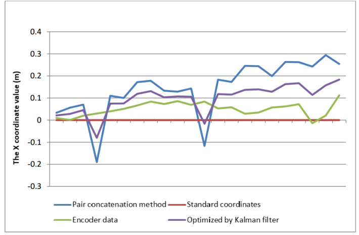 | Figure 17. Statistic of the coordinate values X of the robot |
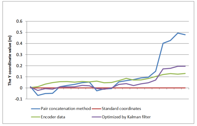 | Figure 18. Statistic of the coordinate values Y of the robot |
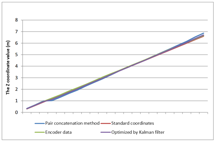 | Figure 19. Statistic of the coordinate values Z of the robot |
4.5.3. Experimental Results of Improved 3D Clouds at Different Room Angles during Robotic Movements
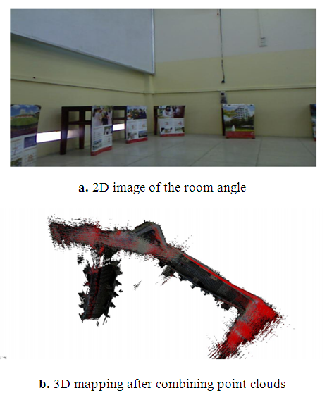
- Figure 20 describes 2D images captured on the robotic pathway in the room environment. The robot moves along the paths to the left and to the right of the room. Therefore, these 2D images of the environment are converted into 3D clouds and then they are grafted to create the 3D spatial images as shown Figure 21, Figure 22 and Figure 23, which show three 3D cloud maps with the paths at different angles.3D cloud mappings with the high accuracy at different room angles are shown using the optimized transformation matrix when the robot moves around.
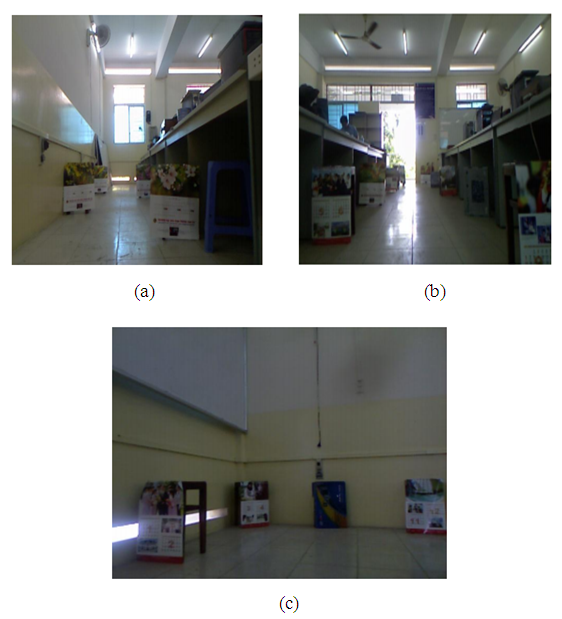 | Figure 20. 2D maps during robotic movements for 3D loud mapping: (a)-Robot moving straight at the room left; (b)- Robot moving straight at the room right; (c)-A room angle |
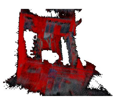 | Figure 21. 3D map of the robot path with the first angle using Kalman filter |
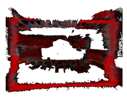 | Figure 22. 3D map of the robot path with the second angle using Kalman filter |
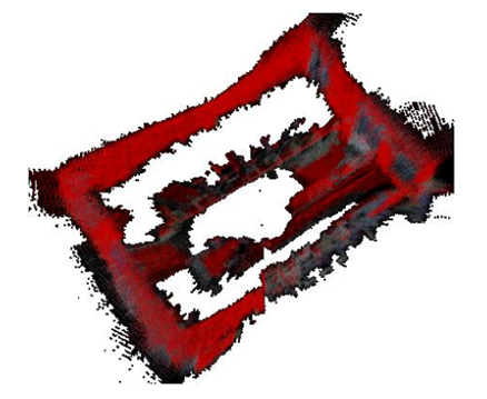 | Figure 23. 3D map of the robot path with the third angle using Kalman filter |
5. Conclusions
- In the paper, the model of mobile platform (robot) in the indoor environment was represented and 3D point clouds were completely reconstructed based on RGB-D image frames obtained from the Kinect camera system. A SIFT algorithm was employed to detect and to describe image features. In addition, encoder data were used to combine to RGB image data and the Kalman filter was utilized to produce the optimized transformation matrix for minimize the cumulative error for robot localization. Experimental results prove that the effectiveness of combining between the Kinect camera system and the encoder sensors on the robot. Moreover, the Kinect can be cheaper cost computation compared to other stereo cameras for indoor applications.
ACKNOWLEDGEMENTS
- This work is supported by HoChiMinh City University of Technology and Education (HCMUTE) under Grant T2017-60TD. We would like to thank HCMUTE, students and colleagues for supports on this project.