-
Paper Information
- Paper Submission
-
Journal Information
- About This Journal
- Editorial Board
- Current Issue
- Archive
- Author Guidelines
- Contact Us
American Journal of Signal Processing
p-ISSN: 2165-9354 e-ISSN: 2165-9362
2018; 8(1): 1-8
doi:10.5923/j.ajsp.20180801.01

Performance Evaluation of Various Hyperspectral Nonlinear Unmixing Algorithms
 Abstract
 Reference
 Full-Text PDF
 Full-text HTML
Awabed Jibreen1, Nourah Alqahtani2, Ouiem Bchir1
1Department of Computer Science, College of Computer and Information Sciences, King Saud University, Riyadh, Saudi Arabia
2Department of Information Systems, College of Computer and Information Sciences, King Saud University, Riyadh, Saudi Arabia
Correspondence to: Awabed Jibreen, Department of Computer Science, College of Computer and Information Sciences, King Saud University, Riyadh, Saudi Arabia.
| Email: |  |
Copyright © 2018 Scientific & Academic Publishing. All Rights Reserved.
This work is licensed under the Creative Commons Attribution International License (CC BY).
http://creativecommons.org/licenses/by/4.0/

Nonlinear unmixing of hyperspectral images has shown considerable attention in image and signal processing research areas. Hyperspectral unmixing identifies endmembers spectral signatures and the abundance fractions of each endmemeber within each pixel of an observed hyperspectral scene. Over the last few years, several nonlinear unmixing algorithms have been proposed. This paper presents an empirical comparison of several popular and recent algorithms of supervised nonlinear unmixing algorithms. Namely, we compared Kernel-based algorithms, graph Laplacian regularization algorithm, and nonlinear unmixing algorithm using a generalized bilinear model (GBM). These unmixing algorithms estimate the abundances of linear, bilinear and intimate mixtures of hyperspectral data. We assessed the performance of these algorithms using Root Mean SquareError on the same data sets.
Keywords: Hyperspectral imagery, Unmixing, Linear model, Nonlinear model, Graph Laplacian regularization, GBM
Cite this paper: Awabed Jibreen, Nourah Alqahtani, Ouiem Bchir, Performance Evaluation of Various Hyperspectral Nonlinear Unmixing Algorithms, American Journal of Signal Processing, Vol. 8 No. 1, 2018, pp. 1-8. doi: 10.5923/j.ajsp.20180801.01.
Article Outline
1. Introduction
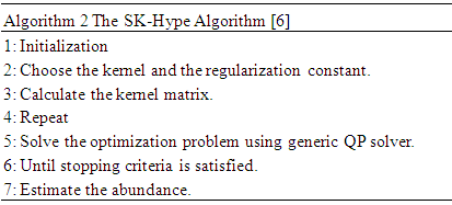
- Hyperspectral image is a three-dimensional data cube which consists of one spectral and two spatial dimensions. Each pixel in the hyperspectral image is represented by a vector of reflectance values (also known as the pixel’s spectrum) whose length is equal to the number of spectral bands considered. Thus, the pixel’s spectrum corresponding to a sole material (such as soil, vegetation, or water) characterizes the material and it is called endmember. Hyperspectral sensors generate high spectral resolution images, but they have a low spatial resolution, which causes mixed pixels within hyperspectral images. As another cause for mixed pixels is a homogeneous combination of different materials in one pixel. Therefore, the hyperspectral spectrum can be seen a mixture of the spectra of each component in the observed scene. This has lead up to linear mixing model and nonlinear mixing model.In fact, the mixing model related to spectral unmixing imagery can be either linear or nonlinear, and that depends on the nature of the observed hyperspectral image. As the photons hit the detector coming from the source, the imaging system bins the observed photons according to their spatial location and wavelength [27]. Linear mixtures are used in case that the detected photons interact mainly with a single component of the observed scene before they reach the sensor. On the contrary, nonlinear mixture models are used when the photons interact with multiple components [4].There are two types of nonlinear mixing: intimate mixing and bilinear mixing. In bilinear mixing, effects of multiple light scattering occur, i.e. the solar radiation scattered by a given material reflects off other materials prior reaching the sensor. In intimate nonlinear mixing, interactions occur at a microscopic level and the photons interact with all the materials concurrently as they are scattered [5, 6].The mixture problem can be solved by applying an appropriate unmixing process. Hyperspectral unmixing is an important process in many fields such as agriculture, geography and geology. It has different applications such as surveillance applications, earth surfaces analysis application, pollution monitoring applications. Spectral unmixing is widely used for analyzing hyperspectral data. It includes two main steps. The first step is determining the pure components in the hyperspectral image (Endmembers). The second step is finding out these materials’ abundances. Spectral unmixing can be either supervised unmixing or unsupervised unmixing. In supervised unmixing, the number of endmember is known while in unsupervised unmixing the number of endmemeber is unknown. Depending on the mixing type, the unimixing processes could be linear and nonlinear.Linear spectral unmixing is to determine the relative proportion (abundance) of materials that are presented in hyperspectral imagery based on the spectral characteristics of materials. The reflectance at each pixel is assumed to be a linear combination of the reflectance of each material (or endmember) existing in the pixel. Linear unmixing methods are used only with the linear mixing models [1].Linear unmixing models cannot handle nonlinear mixing pixels. There are many algorithms and researches regarding linear unmixing, which assumes that pixels are linearly mixed by material signatures weighted by abundances. Recently, nonlinear unmixing for hyperspectral images is receiving attention in remote sensing image exploitation [6] [20] [4] and [18]. Alternative approximation approaches have been proposed for handling the effects of nonlinearity leading to utilizing physics-based nonlinear mixing models [1]. The bilinear mixture model (BMM), has been studied in several researches which is used with second-order scattering of photons between two different materials [8].In this paper, we consider a set of latest and well-known algorithms of supervised nonlinear unmixing of hyperspectral images. We compare empirically these algorithms using the same set of data. The performance is assessed in terms of accuracy.Namely, we compare kernel-based algorithms [6], regularization algorithms [20], and nonlinear unmixing using a generalized bilinear model (GBM) [4]. These unmixing algorithms estimate the abundances of linear, bilinear and intimate mixtures of hyperspectral data. More specifically, for Kernel-based methods we used the K-Hype [6] and Multiple Kernel Learning (SK-Hype) [6] algorithms. For Graph Laplacian Regularization approaches, we considered GLUP-Lap [20] (Group Lasso with Unit sum, Positivity constraints and graph Laplacian regularization) [20]. The outline of the rest of the paper is as follows: The state-of-the-art literature of different general approaches used for solving the hyperspectral unmixing problem is given in section 2. A description of well-known nonlinear unmixing algorithms is provided in section 3. Experimental results and discussion are highlighted in section 4. Conclusion is reported in section 5.
2. Nonlinear Unmixing Approaches
- Yoann Altmann et. al. [19] proposed a nonlinear unmixing method which is based on the Gaussian process. In [19], the abundances of all pixels are identified first, and then the endmembers are estimated using Gaussian regression. They consider a kernel-based method for unsupervised spectral unmixing based on the Gaussian latent variable model (GP-LVM) [29] which is a nonlinear dimension reduction method that has the ability to accurately model any nonlinearity.Jie Chen et. al. [6] addressed the abundances estimation problem of the nonlinear mixed hyperspectral data. They propose a solution to an appropriate kernel-based regression problem. They propose the K-Hype mixture model which is a kernel-based hyperspectral mixture model. They also suggest associated abundance extraction algorithms. The disadvantage of k-Hype is that the balance between linear and nonlinear interactions is fixed. To manage this limitation they propose SK-Hype, which is a natural generalization of K-Hype. It depends on the Multiple Kernel Learning concept. Also, it can automatically adapt between linear and nonlinear contributions. Rita Ammanouil et. al. [20] proposed a graph Laplacian regularization in the hyperspectral image unmixing. The proposed method depends on the construction of a graph representation of the hyperspectral image. Similar pixels are connected by edges both spectrally and spatially. Convex optimization problem is solved using the Alternating Direction Method of Multipliers (ADMM). Graph-cut methods are proposed in order to reduce the computational burden. Yoann Altmann et. al. [18] suggested a Bayesian and two least squares optimization algorithms for nonlinear unmixing. These algorithms assumed that the pixels are mixed by a polynomial post-nonlinear mixing model. They also proposed in [4] a generalized bilinear Method (GBM) where a Bayesian algorithm is proposed to estimate the nonlinearity coefficients and the abundances values.Chang Li et. al. [30] propose a general sparse unmixing method (SU-NLE) that depends on the estimation of noise level. They used the weighted approach in order to provide the matrix of the noise weighting. The proposed approach [30] is robust for different noise levels in different bands of the hyper spectral image. Xiaoguang Mei et. al. [31] propose two methods for nonlinear unmixing of HIS. Robust GBM (RGBM) [32] and another new unmixing method with superpixel segmenta- tion (SS) and low-rank representation (LRR) unmixing approach. In this paper, we empirically compare four nonlinear unmixing algorithms. Namely, we assess the performance of the Kernel-Based Hyperspectral Unmixing Algorithms: the K-Hype Algorithm [6], the Super K-Hype (SK-Hype) Algorithm [6], the Group Lasso with Unit sum, Positivity constraints and graph Laplacian regularization (GLUP-Lap) [20], and the Generalized Bilinear Model (GBM) applied [4].
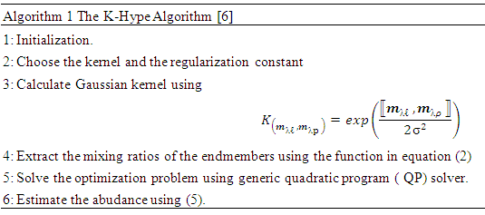
2.1. The K-Hype Algorithm
- The K-Hype [6] is designed for both linear and nonlinear mixing models. It is based on the model defined in (1).
 | (1) |
 is the polynomial kernel of degree 2, m is endmember spectra. R is the number of endmembers.
  is an endmember spectral signature,
  is the
  -th (1XR) row of M Endmember matrix. The constants 1/R2 and 1/2 serve the purpose of normalization. It optimized using quadratic programming.Jie Chen et al. [6] define the function in equation (2) to extract the mixing ratios of the endmembers.
 | (2) |
 is a given functional space,
  is a small positive parameter that controls the trade-off between regularization.
  is unknown nonlinear function that defines the interactions between the endmembers in matrix.
  is dominated by a linear function.This function is defined by a linear trend parameterized by the abundance vector
  , combined with a nonlinear fluctuation term:
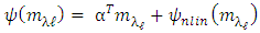 | (3) |
 .where
  can be any real-valued functions on a compact
  of a reproducing kernel Hilbert space
  . The corresponding Gram matrix K is given by:
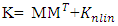 | (4) |
 is the Gram matrix associated with the nonlinear map
  , with
  -thentry
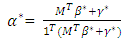
 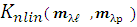 The abundance vector can be estimated as follows:
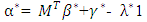 | (5) |
2.2. The SK-Hype Algorithm
- The SK-Hype algorithm [6] is designed for both linear and nonlinear mixing models. The model in equation (3) has some limitations in that the balance between the linear component
 and the nonlinear component
  cannot be tuned. As for K-Hype [6], the Gaussian kernel and the polynomial kernel were considered. Another difficulty in the model of equation (3) is that it cannot captures the dynamic of the mixture, which requires that r or the
  ’sbe locally normalized. Thus Gram matrice is considered as in equation (6)
 | (6) |
 | (7) |
2.3. GLUP-Lap Algorithm
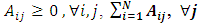
- GLUP-Lap [20] stands for Group Lasse with Unit Sum, Positivity constraint and Laplacian regularization [20]. GLUP-Lap approach [20] is graph based. If two nodes are connected, then they are likely to have similar abundances. They incorporate this information in the unmixing problem using the graph Laplacian regularization. This leads to a convex optimization problem as defined in (8).
 | (8) |
 where
where  is the graph Laplacian matrix given by
  , D is diagonal matrix with
 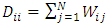 , μ≥0 and λ≥0 are two regularization parameters. The relevance of the regularization are expressed as in (9).
 | (9) |
 , is the degree of similarity. The regularization parameter λ in (8) controls the extent to which similar pixels estimate similar abundances. R is a large dictionary of endmembers, and only few of these endmembers are present in the image.
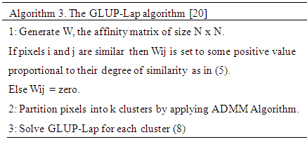 The first and second term of the cost function in (8) can be grouped in a single quadratic form. However the resulting Quadratic Problem has N × M non-separable variables. Its solution can be obtained using the Alternating Direction Method of Multipliers (ADMM) [21]. The GLUP-Lap algorithm steps are described in Algorithm 3.
2.4. GBM Algorithm
- The GBM in [4] assumes that the mixture problem can be expressed as
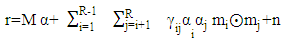 | (10) |
 | (11) |
 Where
Where  is a coefficient that determines the interactions between endmembers #i and #j in the observed pixel. The unknown parameter vector θ that associated with the GBM [4] includes the nonlinearity coefficient vector γ = [γ1,2, . . . , γR−1,R]T, the abundance vector α, and the noise variance σ2.
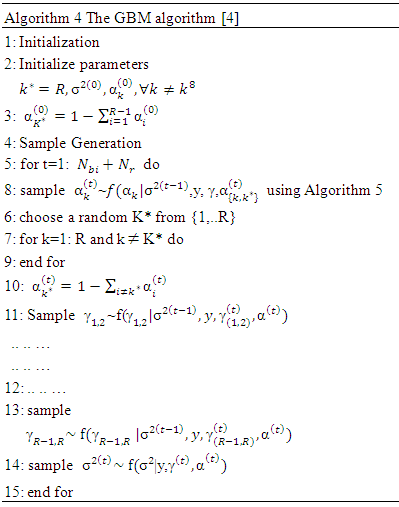 The hierarchical Bayesian model is used to calculate the unknown parameter vector θ= (αT , γT, σ2)T that is associated with the GBM [4]. Metropolis-within-Gibbs algorithm is also used in order to generate sample distribution according to the posterior distribution f(θ|y). The generated samples are then used to estimate the unknown parameters. Metropolis-within-Gibbs algorithm is described in algorithm 5.
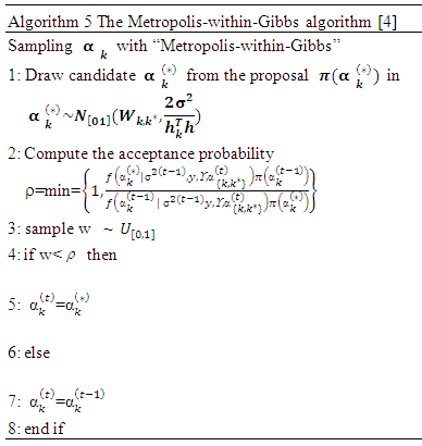
3. Experiments
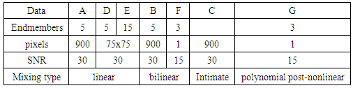
- In this paper, we compare empirically four supervised unmixing algorithms; The K-Hype Algorithm, Super K-Hype (SK-Hype) Algorithm [6], GLUP-Lap [20], and the GBM Algorithms [4]. We use the same endmemer sets and the mixing models that have been used to experiment the considered unmixing approaches as reported in [4], [6], [18], [20]. and [24]. We should mention that these approaches did not use the same data. However, in our experiment, we convey the same data as input to all unmixing approaches in order to compare their performances. Thus, we used 7 input data with different mixture model, number of endmembers, number of signatures (spectra), number of pixels, Signal to Noise Ratio SNR, and abundances. In the follwing, we describe these datasets.Data A is a synthetic image data with 900 pixels that are mixed by linear mixing model using the endmembers, the abundances in [6]. The linear mixing model is defined as:
 | (12) |
 | (13) |
 | (14) |
 | (15) |
 | (16) |
 | (17) |
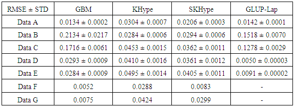
 denotes the Hadamard (term-by-term) product, M is the endmember matrix, a is the abundance and n is the noise. Note that the resulting PPNMM includes bilinear terms. However, the nonlinear terms are characterized by single amplitude parameter b. Table 1 summarises the characteristics of the used data sets.
|
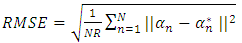 | (18) |
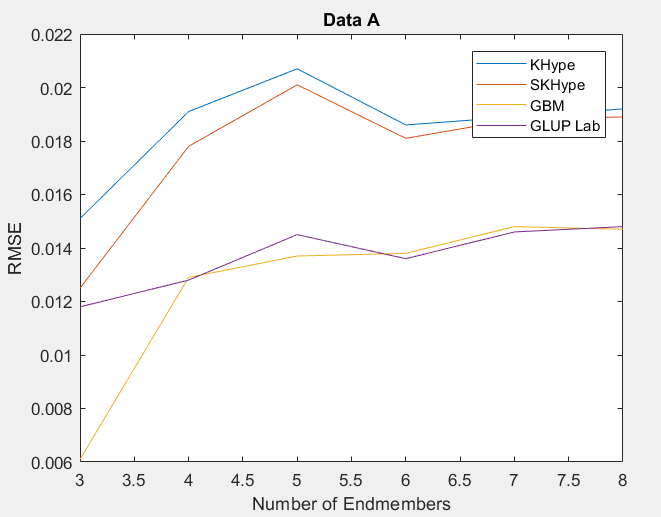 | Figure 1. RMSE of Unmixing Data Awhen varying the number of endmembers |
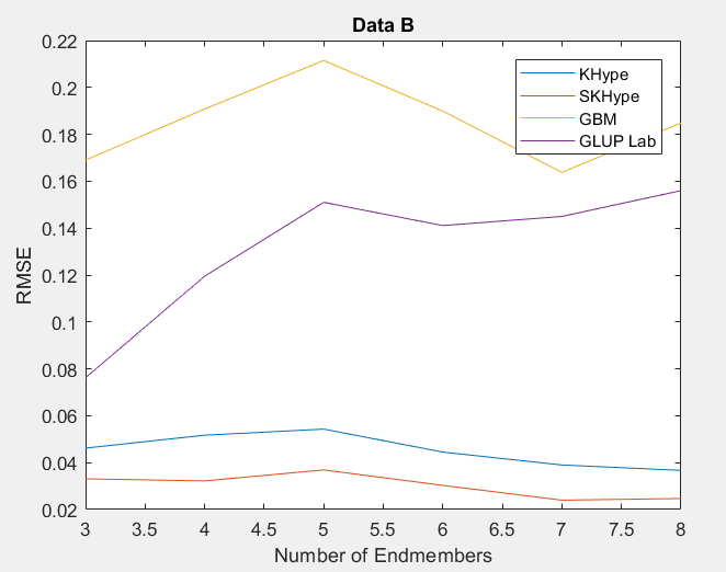 | Figure 2. RMSE of Unmixing Data Bwhen varying the number of endmembers |
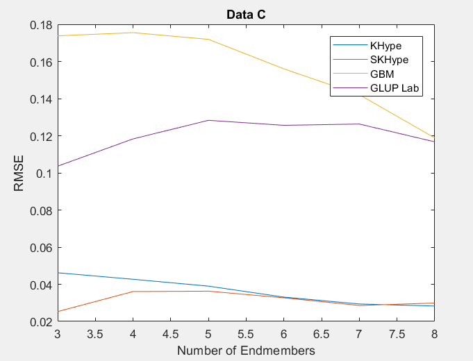 | Figure 3. RMSE of Unmixing Data Cwhen varying the number of endmembers |
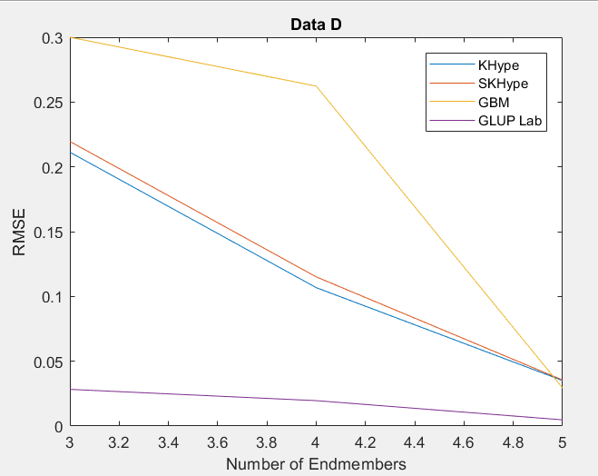 | Figure 4. RMSE of Unmixing Data Dwhen varying the number of endmembers |
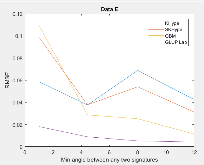 | Figure 5. RMSE of Unmixing Data Ewhen varying the angle between any two signature |
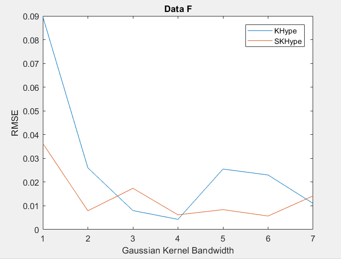 | Figure 6. RMSE of Unmixing Data F when varying the Gussian Kernel bandwith |
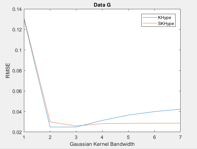 | Figure 7. RMSE of Unmixing Data G when varying the Gaussian Kernel bandwith |
|
|
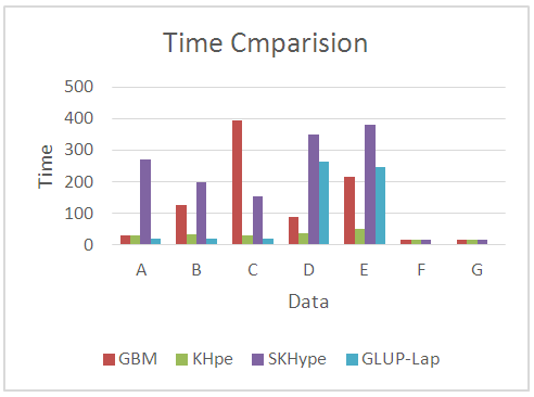 | Figure 8. Time Comparison of the Considered Unmixing approaches |
4. Conclusions
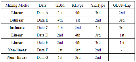
- In this paper, we compared empirically a set of non-linear unmixing algorithms. Seven input data sets have been mixed using different mixing models. The results show that GBM [4] is able to unmix linear and non-linear mixed models. However, it is not able to unmix bilinear or intimate mixed models. On the other hand, KHype [6] and S-KHype [6] give better performance results on bilinear and intimate unmixing models while they are not unmixing linear and non-linear mixing models. Thus, there is no universal unmixing approach that is able to unmix all the considered scenarios. As the performance varies with respect to the data and therfore it is difficult to decide on the unmixing approach to adopt, we plan as future work to investigate combining fusion techniques on these approaches in order to obtain betterunmixing result regardless of the data set. We aim also to consider more approaches and other data sets.