-
Paper Information
- Paper Submission
-
Journal Information
- About This Journal
- Editorial Board
- Current Issue
- Archive
- Author Guidelines
- Contact Us
American Journal of Signal Processing
p-ISSN: 2165-9354 e-ISSN: 2165-9362
2017; 7(1): 1-11
doi:10.5923/j.ajsp.20170701.01

Trilinear Interpolation Algorithm for Reconstruction of 3D MRI Brain Image
 Abstract
 Reference
 Full-Text PDF
 Full-text HTML
Cam Q. T. Thanh, Nguyen T. Hai
Faculty of Electrical and Electronics Engineering, HCMC University of Technology and Education, Ho Chi Minh City, Vietnam
Correspondence to: Nguyen T. Hai, Faculty of Electrical and Electronics Engineering, HCMC University of Technology and Education, Ho Chi Minh City, Vietnam.
| Email: |  |
Copyright © 2017 Scientific & Academic Publishing. All Rights Reserved.
This work is licensed under the Creative Commons Attribution International License (CC BY).
http://creativecommons.org/licenses/by/4.0/

Medical image processing to support doctors for exact diagnosis and early treatment plays an important role. In this paper, construction of a three-dimensional (3D) image from 2DMRI cortex images is proposed. In addition, the 3D image may represent the visual details of brain inside human cortex. The 2DMRI cortex images are pre-processed using the mean filer for removing multiplicative noises and the histogram equalization for enhancement is applied. In addition, the multilevel Otsu method is employed to separate brain part inside the human cortex and a proposed algorithm of the trilinear interpolation is utilized for the construction of a 3D image. Simulation results show that the effectiveness of the proposed approach and also it is a sharing information for developments of 3D image construction.
Keywords: MRI brain image, 3D Construction, Multilevel Otsu and Region Growing, Trilinear interpolation
Cite this paper: Cam Q. T. Thanh, Nguyen T. Hai, Trilinear Interpolation Algorithm for Reconstruction of 3D MRI Brain Image, American Journal of Signal Processing, Vol. 7 No. 1, 2017, pp. 1-11. doi: 10.5923/j.ajsp.20170701.01.
Article Outline
1. Introduction
- Medical image diagnosis plays an increasingly important role in modern medicine. In addition, detection and diagnosis of early potential risks causing cancer for treatment easier is necessary and less costly. In practice, there are many diagnostic imaging techniques such as Positron Emission Tomography (PET), Computed Tomography (CT) Scanner, Magnetic Resonance Imaging (MRI) [1-3].There have been many researches about the process of building 3D images from 2D medical images in recent years. The 3D surface of the knee or a 3D spine image was constructed from 2D CT images [1, 2] using Marching Cube. This method allows to divide data blocks into cubes and each cube was made up of eight adjacent voxels. From these eight adjacent voxels, material surfaces were built using the triangular mesh. Therefore, the method has the advantage of fast calculation, simple construction operations and produces 3D images with the high resolution. However, the calculation will be slow, if one processes the large number of 2D image data. In addition, the images captured from sensors often have noise, because to improve the quality of constructing a 3D image, 2D images need to be pre-processed to reduce noise. In particular, a mean-unsharp filter may be applied to enhance high frequency components and filtered noise.Enhancement method of MRI images [3] was employed by processing the intensity values of grayscale image before low-level image separation. Therefore, low-contrast images may be converted to images with higher contrast. Moreover, morphological operations are often used to make the tumor boundary. In this paper, morphological operations are utilized to allow to stretch and then fill the object for segmentation. The segmentation of image is an important step to build 3D image. Otsu method is often applied to find the gray level threshold values to segment 2D images for construction of 3D image [4, 5]. In this research, the Otsu algorithm will allow to determine an appropriate threshold for segmentation of 2D MRI images [6].A segmentation method is often used in identifying tumors or in building 3D images. An algorithm of regional development was combined with the segmentation method based on the similarity of adjacent pixels with the nuclear point [7]. The result of the combined algorithm depends very much on choosing where the nuclear initial point and the error between the nuclear point and neighboring pixels. In practice, the process of 2D medical image acquisition may appear noise on it. Therefore, a threshold of the traditional Otsu method may be employed to segment some areas for building 3D image. However, this method may lead to the poor result. For the better results, an Otsu method with multilevel are applied to divide 2D image into many layers. Pixels in 2D image have the same regions combined with algorithm of region development [8] to segment the image. The 2D image after segmentation may be processed in the coordinate axes (x, y, z). In particular, linear interpolation algorithm is utilized to construct the 2D image surface by calculating the approximate value of a point between two consecutive layers in the spatial domain [9, 10].This article has the main sections. In particular, Section-I introduces the necessity of building a 3D image based on 2D MRI images and some relevant techniques. In Section-II, the paper will present the image pre-processing problems such as image segmentation, region development for 3D construction. Section-III describes results and discussion. Finally, the conclusion is presented in Section-IV.
2. Materials and Methods
- Dataset with 44 2D MRI brain images with 256x192 pixels, which are provided by Binh Duong General Hospital, are used for construction of 3D image in this research.3D image construction from 2D MRI human cortex images will be performed the following steps as described in Figure 1. Firstly, the 2D MRI images are pre-processed, including noise rejection and image enhancement. The second is that the morphological operator is employed in order to remove pixels around boundaries of objects in the 2D images. Thus, the pre-processed images are segmented for the purpose of separating the brain area from the cortex for 3D construction. Finally, the 2D images after the segmentation will be constructed to produce the 3D image using a trilinear interpolation algorithm as shown in Figure 1.
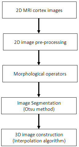 | Figure 1. Block diagram of 3D image construction |
2.1. Image Pre-processing
- For constructing 3D image, 2D MRI images with noise are smoothed using an average filter. This average filter is convoluted with each 2D MRI image to remove noise using the following equation:
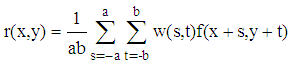 | (1) |
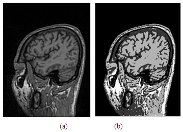
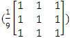 . Thus, the convoluted image is processed to be smoother and it also retains the complete brain region after separating from the cortex image compared with the image using the median filter as shown in Figure 3.
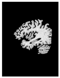
 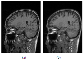 | Figure 2. (a)-Original human cortex image; (b)-Cortex image after the mean filter |
 | Figure 3. (a)-image after using the mean filter; (b)-image after using the median filter |
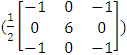 is applied to remove the low frequency components and to enhance the image with the high frequency components as shown in Figure 4.
 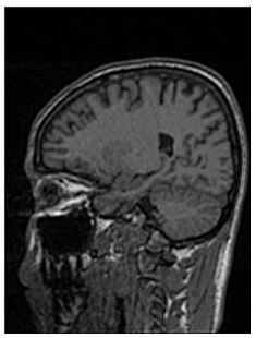 | Figure 4. 2D MRI cortex image after the unsharp filter |
 | (2) |
 | (3) |
 | Figure 5. (a)-Image using the unsharp filter; (b)-Image after enhancement |
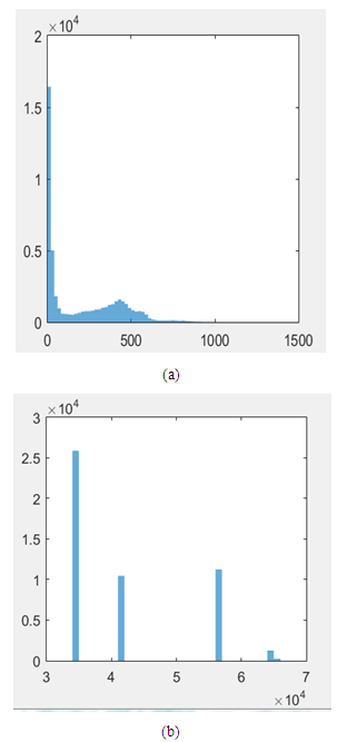 | Figure 6. Representation of images: (a)-Image before enhancement; (b)-Image after enhancement using the histogram equalization |
2.2. Morphological Operation
- After filtering 2D MRI cortex image to remove noise and then enhancing it, the enhanced image is processed for imperfection of the image. Therefore, a morphological algorithm is applied to remove some parts which are not necessary around objects in the image. In particular, the image using the morphological algorithm just retains the important object for construction of 3D image. In particular, in the morphological operations including Dilation and Erosion, the dilation operator is employed to process the 2D enhanced image based on its shapes and structures. In this case, the morphological operation is used to combine boundaries of objects and to remove the undesired parts around the objects [12]. For image calculation, the morphological image is performed by convoluting between the input image and a kernel as follows:
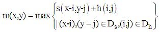 | (4) |
 | Figure 7. Structuring matrix of the 2x2 kernel |
 | Figure 8. (a)-Representation of the enhanced image; (b)-Image after the morphological operation |
2.3. Otsu Method for Image Segmentation
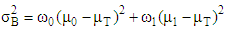
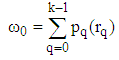
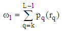
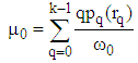
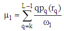
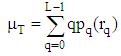
- Image segmentation plays an important role in constructing a 3D medical image. In this research, all slices of 2D brain images are segmented before construction. An Otsu algorithm is employed for these 2D MRI image segmentation. In particular, this algorithm allows to calculate many gray level thresholds and the threshold value is chosen corresponding to the minimum variance within the class. The segmentation algorithm for the set of 2D MRI cortex images is expressed as flows:
 | (5) |
 | (6) |
 | (7) |
 | (8) |
 | (9) |
 | (10) |
 | (11) |
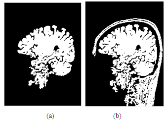
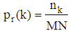
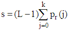
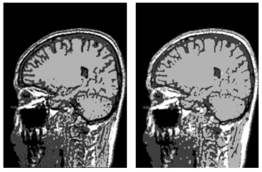
 are the background and foreground variances, pr(rq) describes the probability density function of the image histogram.Figure 8 shows the result of the 2D cortex image after segmentation using the traditional Otsu method from the morphological image in Figure 8(b). In the segmentation using the traditional Otsu method with the 7 thresholding, the image has advantages of making the quick segmented image. However, the segmentation of this traditional method completely depends on a threshold based on the minimum variance, so the segmented image may make the undesired object with some lost parts as the blue circle shown in Figure 9.
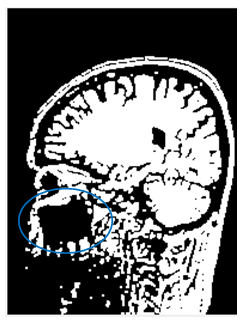 | Figure 9. MRI cortex image segmented using the traditional Otsu method with the 7 thresholding |
 | Figure 10. (a)-Original image; (b)-image after the traditional Otsu segmentation |
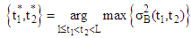 | (12) |
 are two thresholds chosen corresponding to the maximum variance within the class. Figure 11 shows the simulation result of the segmented image using the traditional Otsu method with two thresholds, in which the mouth object in this image is seen more clearly compared to that in Figure 9.
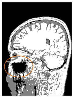 | Figure 11. Representation of the 2D MRI cortex segmented using the Otsu method with two multilevel |
 | (13) |
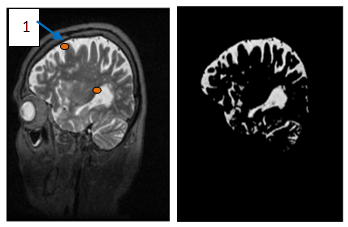 | Figure 12. (a)-Enhanced image, (b)-Brain object after segmentation combined with the region growing corresponding to the seed positioned at point-1 |
 | Figure 13. (a)-Enhanced image, (b)-Brain object after segmentation combined with the region growing corresponding to the seed positioned at point-2 |
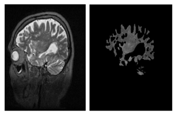
 | Figure 14. Representation of the processed images, in which (a)-the enhanced image; (b),(c),(d)-Images after segmentation with seed positioned at points 1, 2, 3 |
 | Figure 15. Image representation after convolution between the original and the segmented image |
2.4. Interpolation Algorithm for 3D Construction
- A constructed 3D brain image consists of a set of many 2D images, there are 44 image slices in this research. 2D brain images after segmentation are built to overlap in order on a coordinate system (x,y,z) [15-20]. In this paper, the 3D brain image is not only constructed based on 44 2D brain images to view the brain object surface, but also it is constructed to observe problems inside this 3D brain part at different angles. A trilinear interpolation method is employed to calculate pixels between two slices as modelled in Figure 16.
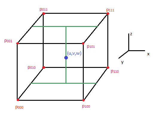 | Figure 16. Representation of a trilinear interpolation model |
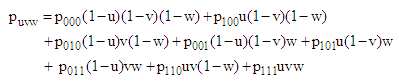 | (14) |
3. Results and Discussions
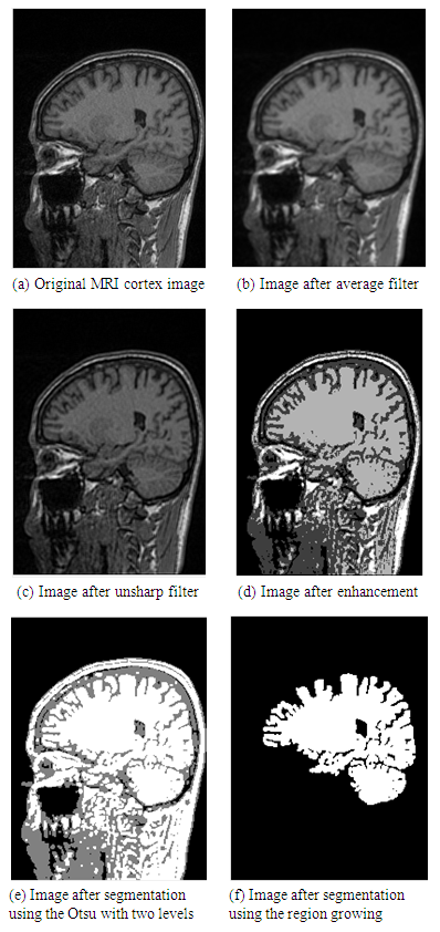
- In this research, a set of 44 MRI cortex images were collected from an MRI machine in Binh Duong General Hospital. The simulation results show that in order to construct a 3D brain image, 2D MRI cortex images need to be processed for enhancement and segmentation of these 2D images as shown in Figure 17 and Figure 18. In the image segmentation, the thresholds with two levels were calculated to produce the desired image.The image is segmented by the Otsu multilevel method as shown in Figure 17(d). The segmented images are continued to process using the region growing method as described in Figure 17(e). It is obvious that the segmented image is the binary image with the pixel values, [0 1]. This 2D image will be used to construct a 3D image with the desired object.Figure 18 shows 12 original MRI cortex images composing of slices 3, 6, 13, 17, 19, 22, 24, 26, 28, 31, 34, 44 of 44 images.Figure 18 represents the simulation results of the segmented images to show the brain objects using the Otsu method with two thresholds combined with the region growing algorithm from 12 MRI cortex images in Figure 17.
 | Figure 17. Representation of the pre-processing image |
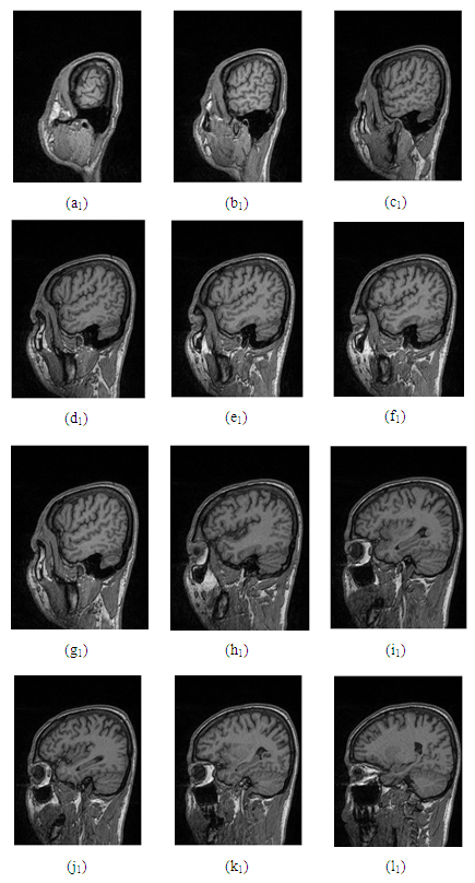 | Figure 18. Representation of the morphological cortex images |
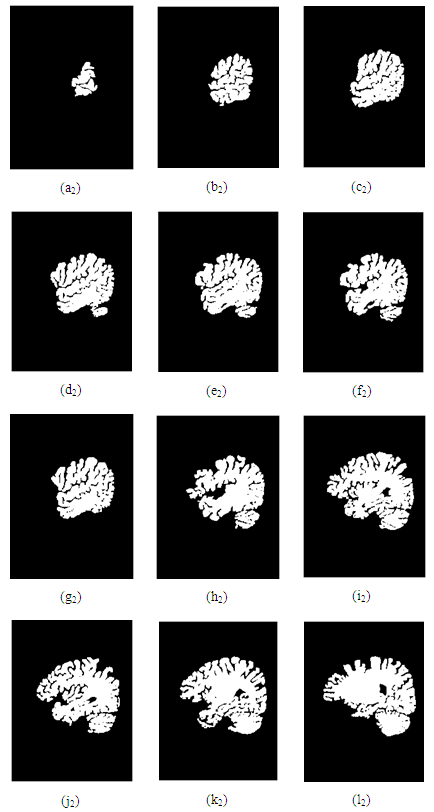 | Figure 19. 12 brain images after segmentation |
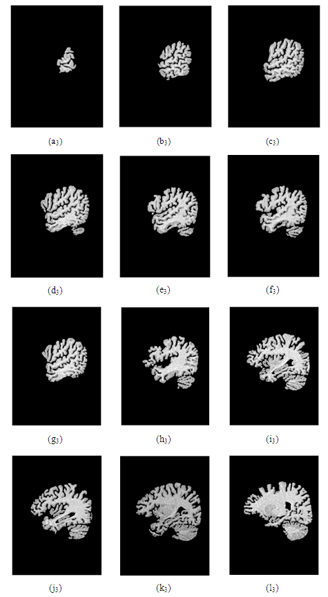 | Figure 20. Images after convolution |
 | Figure 21. The 3D model of brain viewed from different elevations and azimuth angles |
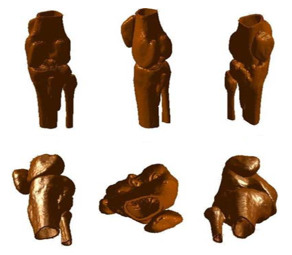 | Figure 22. 3D models of the knee image viewing from different elevations and azimuth angles [2] |
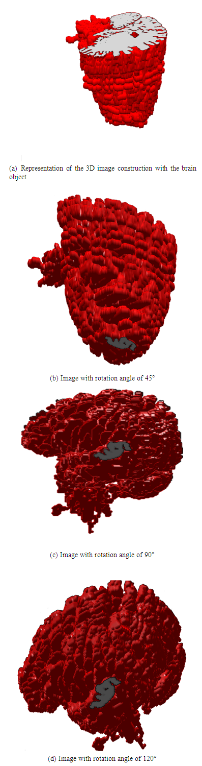
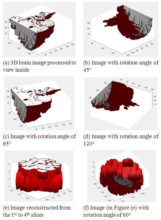 | Figure 23. Representation of the 3D reconstructed image with cutting slices and rotating them |
4. Conclusions
- In this paper, 44 2D MRI cortex images were pre-processed before construction of a 3D brain image. In particular, the brain parts in the 2D cortex images which need to observe at different angles, are separated. From the 2D images, after enhancement of the images using the histogram equalization, the multilevel Otsu method was applied to segment each human cortex image to produce the part of brain for consideration and diagnosis. For observation at different angles of the 3D brain image, the trilinear interpolation method was utilized to construct the 3D brain image from the enhanced 2D MRI images. Simulation results shows that the 3D brain image which allows to view at different angles may support for doctors in early diagnosing problems inside human brain cortex for treatment easier.
ACKNOWLEDMENTS
- The author is highly grateful to Binh Duong General Hospital, where provided MRI image database for this research.