Mohamed B. El Mashade
Electrical Engineering Dept., Faculty of Engineering, Al Azhar University, Cairo, Egypt
Correspondence to: Mohamed B. El Mashade, Electrical Engineering Dept., Faculty of Engineering, Al Azhar University, Cairo, Egypt.
| Email: |  |
Copyright © 2016 Scientific & Academic Publishing. All Rights Reserved.
This work is licensed under the Creative Commons Attribution International License (CC BY).
http://creativecommons.org/licenses/by/4.0/

Abstract
Conventional methods of CFAR detection always use windowing, in the sense that some number of cells are investigated and the target present/absent decision is made according to the composition of the cells in that window. The most desirable version of CFAR schemes is the CA algorithm, given that the background noise is homogeneous. However, the existence of heterogeneities in practical operational environments renders this processor ineffective. In an attempt to overcome this drawback, the strong interferers are censored before carrying out the cell-averaging operation. This is the fundamental procedure of the double-threshold (DT) algorithm which represents one of the most important detectors that has interference immunity against heterogeneous operating environments. It relies on comparing the cells of the reference window to an excision threshold so that only the surviving cells are averaged to yield the needed power estimate of the unknown noise level. Thus, the trimming operation ensures that the calculation of the detection threshold is based on a set of samples which is free of strong interferers and is therefore much more representative of the actual noise level. On the other hand, the target fluctuation model plays an important role in the design and performance evaluation of all radar systems. The Swerling models bracket the behavior of fluctuating targets of practical interest. The correlation coefficient between two consecutive echoes in the dwell-time is equal to unity for SWI & SWIII and is zero for SWII & SWIV models. An important class of targets is represented by the so-called moderately fluctuating χ2 targets with a correlation coefficient in the range 0<ρ<1. Here, our intention is to analyze the performance of the DT-CFAR processor in detecting such type of fluctuating targets in the absence as well as in the presence of outlying targets. Numerical results demonstrate that it is robust in multitarget situations even when more than half of the search region is occupied by spurious target returns.
Keywords:
CFAR detection, χ2 fluctuating targets with 2 & 4 degrees of freedom, SWI-SWIV models, Partially-Correlated targets, Interference-Saturated environment, Noise and clutter, Post-Detection integration
Cite this paper: Mohamed B. El Mashade, Performance Amelioration of Adaptive Detection of Moderately-Fluctuating Radar Targets in Severe Interference, American Journal of Signal Processing, Vol. 6 No. 2, 2016, pp. 32-55. doi: 10.5923/j.ajsp.20160602.02.
1. Introduction
Radars have been used for decades to detect targets for traffic control, air defense, and weather prediction. These targets may be found on the ground, on the sea, in the air, in space, and even below ground. Additionally, radar represents a significant part of air-defense system as well as the operation of offensive missile and other weapons. In air defense, it performs the function of surveillance and weapon control. Surveillance includes target detection, target tracking and designation to a weapon system. On the other hand, the present era of limited warfare demands precision strikes for reduced risk and cost efficient operation with minimum possible guarantee damage. In order to meet such exact challenges, automatic target detection capability is becoming increasingly important to the defense community. Practically, radar is an instrument that is used for observing a natural environment and detecting physical objects herein. It employs electromagnetic waves to illuminate the environment, and receives echoes reflected by the objects. After reception, the signal is processed before it is displayed to the user. The ability to detect objects at long distances, or in conditions of poor visibility, is the key feature of the radar. This is of particular importance for aircrafts and ships in order to navigate safely and avoid collisions. In the illuminated environment, numerous objects may introduce reflection and scattering of the transmitted radar signal, causing difficulties in detecting objects of interest. These objects are usually termed as targets, whilst the interfering echoes are usually termed as clutter. Clutter echoes are random and have thermal noise-like characteristics because the individual clutter components have random phases and amplitudes. In many cases, the clutter signal level is much higher than the receiver noise level. Thus, the radar’s ability to detect targets embedded in high clutter background depends on the signal-to-clutter ratio (SCR) rather than the SNR. While the white noise normally introduces the same amount of noise power across all radar range bins, the clutter power may vary within a single range bin. Since clutter returns are target-like echoes, the only way of distinguishing target returns from clutter echoes is based on the target radar cross section (RCS). Therefore, signal detection in noisy or clutter environments is a very important part of target detection procedure [1-6]. The detection of signals becomes complex when radar returns are from non-stationary background noise (or noise plus clutter). The probability of false alarm increases intolerably when a detection scheme employing a fixed threshold is used. Therefore, adaptive threshold techniques are required in order to maintain a nearly constant false alarm rate. The key factor of CFAR algorithms lies in setting the threshold adaptively by estimating the background noise power included in a test cell. Averaging the outputs of the reference cells surrounding the test cell forms this estimate in the conventional CA detector. This processor is very effective in case of stationary and homogeneous interference and is effective almost as the ideal, Neyman-Pearson, detector when the number of reference cells becomes very large. In a non-homogenous environment, on the other hand, the detection performance and the false alarm regulation properties of CA detector may be seriously degraded. During the last few years, a lot of different approaches have been suggested to ameliorate the heterogeneous detectability of CFAR schemes. The double-threshold (DT) procedure constitutes one of such techniques that maintain a constant rate of false alarm as well as perform well in non-homogeneous environments; especially in multiple-target situations. The trimming threshold ensures that the calculation of the detection threshold is based on a set of samples which is free of strong interferers and is therefore much more representative of the noise level. Even if the trimmer fails to discard all interferers, it nullifies the largest ones amongst them, leaving only those below the trimming threshold. If the trimming threshold is properly set, the impact of the remaining interferers should be tolerable. Owing to the importance of this type of CFAR processors, especially in detecting targets in an interference saturated environments, its performance was analyzed by El_Mashade [7-9] under different cases of operating circumstances. The detection capabilities of radars cannot be assessed without radar cross section (RCS) data for all their potential targets, defined as functions of the target's orientation relative to the radar. In general, RCS is a complex function of aspect angle, frequency, and polarization even for relatively simple targets. Furthermore, received power at the radar (target echo only, not including noise or other interference) is proportional to the target RCS. Thus, RCS fluctuations result in received target power fluctuations. The larger the scatterer separation in terms of wavelengths, the more rapidly the RCS varies with angle or frequency. Because the exact nature of this fluctuation is difficult to predict, a statistical description is often adopted to characterize the target radar cross section. Amongst the statistical models of RCS fluctuation, there are two fundamental density functions: χ2-distribution with 2 and 4 degrees of freedom. SWI and SWIII target models apply when the cross-section fluctuates from scan to scan, where the return signals are highly correlated, that is to say, the pulse repetition rate is high with respect to the target dynamics. Target models SWII and SWIV, on the other hand, stratify when the fluctuation is rapid, from one pulse to the next. The return signals are de-correlated due either to the low pulse repetition rate, with respect to the target dynamics, or to the rapidly changing of the target aspect angle with respect to the pulse repetition frequency [10-12]. Although the Swerling cases bracket the behavior of fluctuating targets of practical interest, recent investigations of target cross section fluctuation statistics indicate that some targets may have probability of detection curves which lie considerably outside the range of cases which are satisfactorily bracketed by the Swerling cases. An interesting class of those targets is that represented by the so-called moderately fluctuating Rayleigh and χ2 targets, which when illuminated by a coherent pulse train, return a train of correlated pulses with a correlation coefficient in the range 0<ρ<1. The detection of this type of fluctuating targets is therefore of significant interest [13-15]. Our goal in the present paper is to analyze the performance of DT-CFAR procedure for partially-correlated χ2-targets with two and four degrees of freedom in the absence as well as in the presence of spurious targets. In section II, we formulate the problem and compute the characteristic function of the post-detection integrator output for the case where the signal fluctuation obeys χ2 statistics with two and four degrees of freedom. Section III is devoted to the performance analysis of the underlined detector in the presence of spurious targets. Section IV deals with the presentation of our simulation results in the absence as well as in the presence of outlying targets. In section V, we present a brief discussion along with our conclusions.
2. Statistical Background and Detector Description
In an automatic radar detection system, the received signal in every range resolution cell is compared with a threshold to test for the presence of a target. For the simple case where the noise is homogeneous, a fixed threshold is adequate to achieve the designed rate of false alarm. In the more realistic case, the noise background is non-stationary due to clutter and interference. In this situation, the threshold used for testing a particular cell is usually set adaptively, using data from nearby resolution cells, to keep a pre-assigned false alarm rate under variations in the noise level. In actual applications, the assumption that no other signals except noise are present in the reference cells is often violated. Beside the legitimate signals, interfering signals originating from wideband jamming noise, jamming pulses and unintentional interferences can be expected. The presence of strong signals (to which we shall refer as interferences) amongst the contents of reference window may have a catastrophic effect on the performance of a conventional CA detector; in particular if these interferences are considerably stronger than the desired signal. This is frequently the case when legitimate signals have a large dynamic range. To combat the presence of such unwanted signals, it is naturally to exclude them from the implementation of the detection threshold. This is actually the function of the trimming threshold in DT detector. This processor suffers almost no degradation in performance, in comparison with the conventional CA detector, when it operates in an environment of homogeneous noise such as thermal noise with the possible addition of wideband jamming [7]. In practice, CFAR detection is often implemented after non-coherent integration, as illustrated in Fig.(1). The echo return of each pulse is detected by a square-law device and the sum of M squared envelopes is used to represent the output of each reference cell. In analog implementation, these cells are obtained from a tapped delay line. The cell under test (CUT) is the central cell whose output "Θ0" is also the sum of M squared envelopes. The immediate neighbors of the CUT are excluded from the CFAR processing due to a possible spillover from the CUT. Whenever the cell being tested changes, the rightmost sample is shifted out and a new sample enters the leftmost side of the register. This updating process proceeds until the maximum unambiguous range is reached. The output of reference cells (N/2 on each side of the CUT) is processed to estimate the unknown noise power level. These reference cells are fed to a censoring process in order to discard any sample the content of which exceeds a predefined threshold "τ". This will ensure that the final detection threshold is free of any interferer returns and consequently it represents the actual background noise level. The surviving samples Θi's, i=1, ….., n, enter an averaging process to estimate the unknown noise level which is used to implement the detection threshold after scaling it with a constant factor "T". Detection of the desired target, in the CUT, is declared if: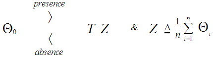 | (1) |
When a target is present, the amplitude of the signal at the receiver depends on RCS, which is the effective scattering area of a target as seen by the radar. In general, the RCS of target fluctuates because targets consist of many scattering elements, and returns from each scattering element vary. When simulating target seekers, there is a great need for computationally efficient target models. Target RCS fluctuations are often modeled according to the four Swerling target cases. These fluctuating models assume that the target RCS fluctuation follows either a Rayleigh or one-dominant-plus Rayleigh distribution with scan-to-scan or pulse-to pulse statistical independence. In Swerling case I (SWI), the echoes are part of a Rayleigh power distribution, and do not fluctuate during a look but fluctuate between looks. Swerling case II (SWII) is as case SWI, with the exception that the echoes fluctuate from pulse to pulse during each look. In SWIII, the echoes are part of a χ2-distribution with four degrees of freedom but instead of fluctuating during a look, it fluctuates between looks. On the other hand, SWIV is similar to SWIII with the exception that the echoes fluctuate from pulse to pulse during each look. Mathematically, these four types of fluctuating targets are based on two RCS distributions and two fluctuation rates according to: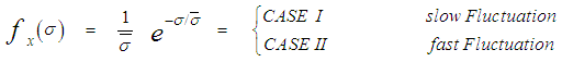 | (2) |
 symbolizes the average cross section over all target fluctuations.
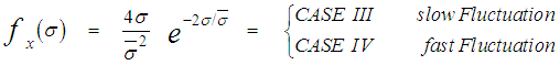 | (3) |
The slow fluctuation case assumes constant RCS during a scan with scan-to-scan variations, while the fast fluctuation case represents target whose returns are independent from pulse-to-pulse.The exact method of prediction of RCS is very complex even for simple and conventional shaped objects. Therefore, the statistical representation is often adopted to characterize it. There are many distribution functions that can be used to depict RCS. The more important one is the so-called χ2-distribution with 2ν degrees of freedom. This model approximates a target with a large reflector and a group of small reflectors, as well as a large reflector over a small range of aspect values. The χ2-family includes the Rayleigh (SWI & SWII) model, the four degrees of freedom model (SWIII & SWIV), the Weinstock model (ν <1) and the generalized model (ν is a positive real number). These models have the property that the distribution is more concentrated about the mean as the value of the parameter ν is increased. Mathematically, this distribution can be formulated as: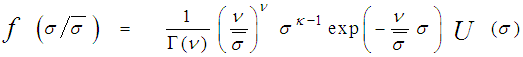 | (4) |
U(.) denotes the unit step function. When ν=1, the PDF of Eq.(4) reduces to the exponential or Rayleigh power distribution that applies to the SWI. On the other hand, SWII, SWIII, and SWIV correspond to ν=M, 2, and 2M, respectively. When ν tends to infinity, the χ2-distribution is constricted to the non-fluctuating target model. If the radar target fluctuates obeying χ2-distribution with κ=2ν degrees of freedom, it can be mathematically represented by a characteristic function (CF) of the form [10]: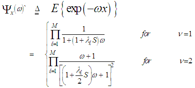 | (5) |
The symbol E{.} in the above formula denotes the expectation operator, S represents the signal-to-noise ratio (SNR), and λi’s symbolize the nonnegative eigenvalues of the correlation matrix "Ω". With review of Eq.(5), it is obvious that the case of partially-correlated demands the computation of λi’s for the processor performance to be evaluated. To achieve this requirement, it is assumed that the signal is statistically stationary and it can be represented by a first order Markov process. Taking these assumptions into consideration, the correlation matrix "Ω" takes the form of definite nonnegative Toeplitz which can be mathematically formulated as [13]: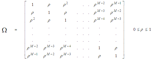 | (6) |
It is required to reformat Eq.(5) in a more simpler form for the processor performance to be easily analyzed. This attractable version takes another easily processed form as: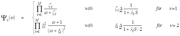 | (7) |
It is of importance to note that the eigenvalues for the SWIII and SWIV (ν=2) target fluctuation models are the same as that for SWI and SWII cases (ν=1), respectively. Eq.(7) is the backbone of our analysis in the current research. For χ2-fluctuation model, the PDF of the output of the ith test tap is given by the Laplace inverse of Eq.(7) after making some minor modifications. If the ith test tap contains noise alone, S must be set to zero (S=0), that is the average noise power at the receiver input is "ψ", which we take it as unity in our analysis without loss of generality. If the ith range cell contains a return from the primary target, it rests as it is without any modifications, where S represents the strength of the target return at the receiver input. On the other hand, if the ith test cell is corrupted by interfering target return, S must be replaced by I, where I denotes the interference-to-noise ratio (INR) at the receiver input.Since the unknown noise power level estimate Z is a random variable, the processor performance is determined by calculating the average values of false alarm and detection probabilities. The probability of adaptive detecting a fluctuating target obeying two degrees of freedom χ2 model is [14]: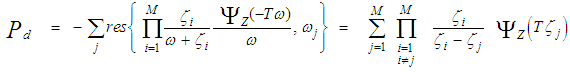 | (8) |
On the other hand, when the fluctuation of the primary target follows χ2- distribution with four degrees of freedom, the probability of detection becomes [15]: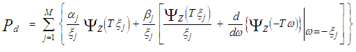 | (9) |
where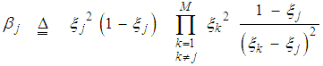 | (10) |
and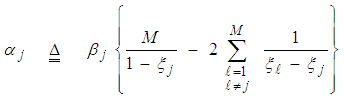 | (11) |
In any situation, the probability of false alarm can be calculated as [8]: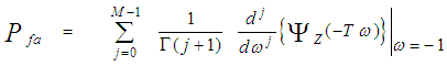 | (12) |
From this relation, it is evident that the backbone of our analysis is the evaluation of the nonnegative eigenvalues of Ω that corresponds to the cell under test variate along with the determination of the CF of the background noise level. This is indeed what we will go to calculate in the next section for the detection performance of the underlined adaptive scheme to be completely analyzed.
3. Heterogeneous Detection Performance of DT Processor
The problem of detecting target signals in background noise of unknown statistics is a common problem in sensor systems. A solution to overcome the problem of noise added to the target signal and to enhance the detectability of targets in these situations is to use adaptive digital signal processing techniques. The key assumption in the CFAR scheme is that the reference cell variates have the same distribution as that of the CUT variate in the no target present case. Therefore, when the reference set variates Θk’s, k=1, 2,….., N, are taken to be square-law detected and non-coherently integrated Gaussian noise variates, they become statistically independent and identically distributed (IID) random variables. These samples pass through a censoring process of threshold "τ", the operation of which is mathematically defined as: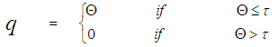 | (13) |
A sample q that was survived is a random variable with a PDF given by: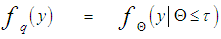 | (14) |
The content of each reference cell has a CF similar to that given in Eq.(7) after setting S equal to zero (S=0). Therefore, the PDF of Θ can be easily obtained by taking the Laplace inverse of the resulting formula. Thus, | (15) |
where L-1 denotes the Laplace inverse operator. The substitution of Eq.(15) into Eq.(14) yields: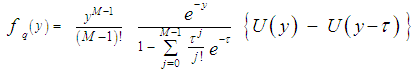 | (16) |
It is seen from Eq.(16) that the PDF of "q" is that of "Θ" truncated at the threshold "τ" and properly normalized. The probability that a sample was not discarded by the trimming process is: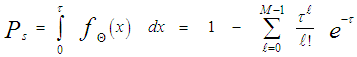 | (17) |
The processor performance is significantly affected when the assumption of homogeneous reference window is violated. There are two major problems that require careful investigation in such scheme of adaptive detection in the case where the operating environment is heterogeneous: regions of clutter power transitions and multitarget situations. The multiple-target case is encountered when there are two or more closely spaced targets in range. This type of environments is frequently encountered in practice where the noise estimate includes the interfering signal power leading to an unnecessary increase in overall threshold and this in turn results in serious degradation in processor detection performance. Since the homogeneous case can be treated as special case of heterogeneous one, we are concerned here with the target multiplicity situation of the processor performance. To analyze the detector performance in the presence of outlying targets, the amplitudes of all targets are assumed to fluctuate according to χ2-model with 2 and 4 degrees of freedom. On the assumption that the sample set contains "ℓ" cells from interfering target returns with interference power ψ(1+I) and "m" cells from clear background with noise power ψ. Without loss of generality, we assume that ψ is unity. The sample mean computed by the detector is [9]: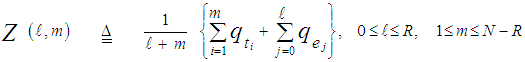 | (18) |
In the above expression, N denotes the length of the shift register and R represents the number of reference cells that are contaminated with outlying target returns, before the censoring process takes place. On the other hand, "m" and "ℓ" denote the number of surviving thermal and interferer samples, respectively, after the application of the discarding process. It assumes that m≥1, but allows ℓ=0 (i.e. all interferer samples are discarded). If m=0, this implies that no samples survived the trimming process and therefore the detection test is suspended. Since the noise and target samples are statistically independent, the sample average Z has a CF given by: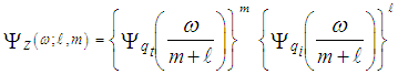 | (19) |
A clutter sample qt that was not excised is a random variable with a PDF given by Eq.(16) whilst that belonging to outlying target has a PDF of the form: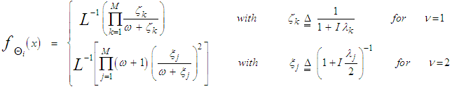 | (20) |
The mathematical treatment of the Laplace inverse transformation will lead to: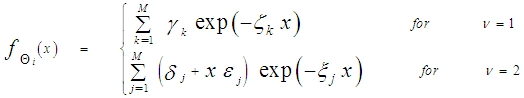 | (21) |
where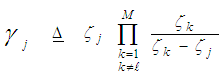 | (22) |
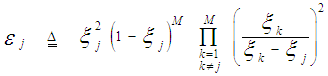 | (23) |
and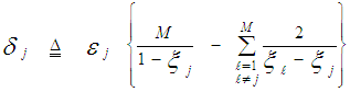 | (24) |
As a function of the PDF of the excisor input, the PDF of its output has a mathematical relation given by: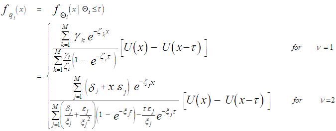 | (25) |
The Laplace transformation of the above formula will result in calculating the CF of the survived cell that associated with the spurious target return. Thus, 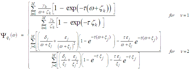 | (26) |
On the other hand, the thermal noise sample has a CF of the form given by: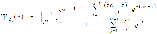 | (27) |
Let Pm(m) and Pℓ(ℓ) denote the probabilities of "m" noise samples and "ℓ" interfering samples surviving the discarding process, respectively, then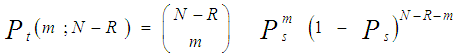 | (28) |
and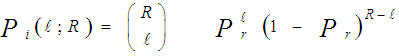 | (29) |
where Ps is as previously defined in Eq.(17). On the other hand, the probability that an interfering sample was not excised by the trimming process is: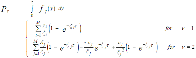 | (30) |
The using of Eq.(30) in Eq.(29) results in finding the probability that "ℓ" outlying samples success to escape from the discarding process. Finally, the conditioning on "m" and "ℓ" is removed by averaging Eq.(19) which leads to: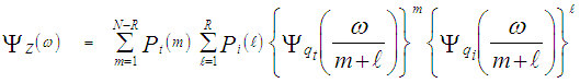 | (31) |
The substitution of Eqs.(26-29) into the above formula gives the CF of the noise level estimate when the primary as well as the secondary outlying targets fluctuate following χ2-distribution with two degrees of freedom. The mathematical processing of these equations yields: 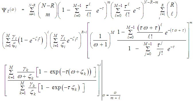 | (32) |
For fluctuating targets corresponding to χ2-statistics with four degrees of freedom, on the other hand, Eq.(31) becomes: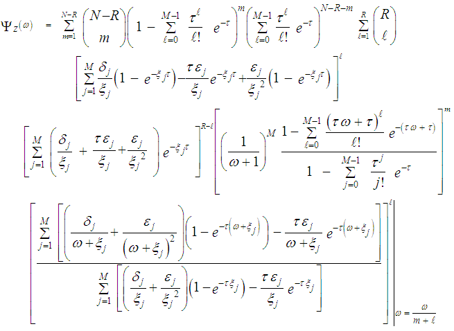 | (33) |
Once the CF of the noise power estimate is obtained, the processor detection performance is completely determined since this function represents the backbone of its calculation either the target under test fluctuates following χ2-statistics with two degrees of freedom or its fluctuation obeying χ2-distribution with four degrees of freedom as Eqs.(8-9) demonstrate. Now, we are in a position that enables us to carry out some numerical results to obtain an idea about the behavior of the double-threshold detector against the presence of partially-correlated χ2 fluctuating targets amongst the contents of the estimation set when the researching along with the secondary interfering targets reflects correlated returns, in accordance with χ2-statistics of 2 and 4 degrees of freedom, to the radar receiver. The displayed numerical values provide some insight into the impact of the various parameters on the detector performance and therefore assist in the design of proper determination of the processor characteristics.
4. Processor Performance Assessment
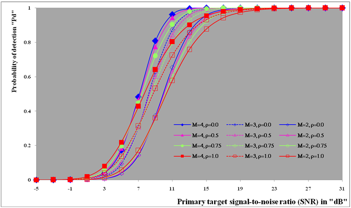
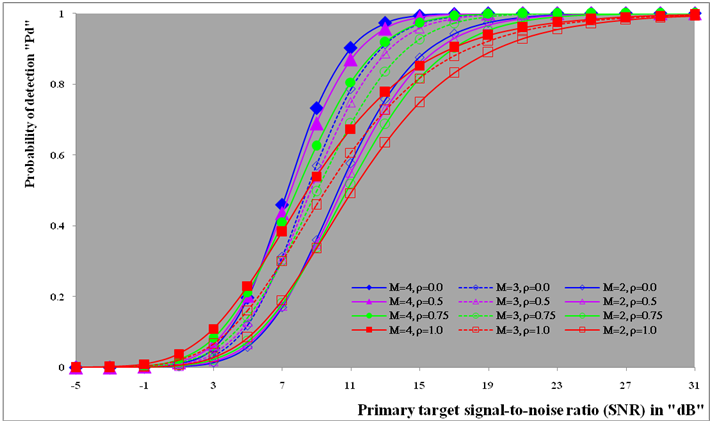
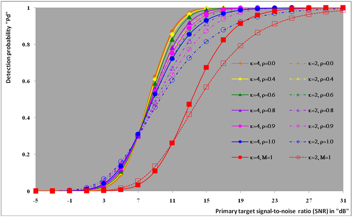
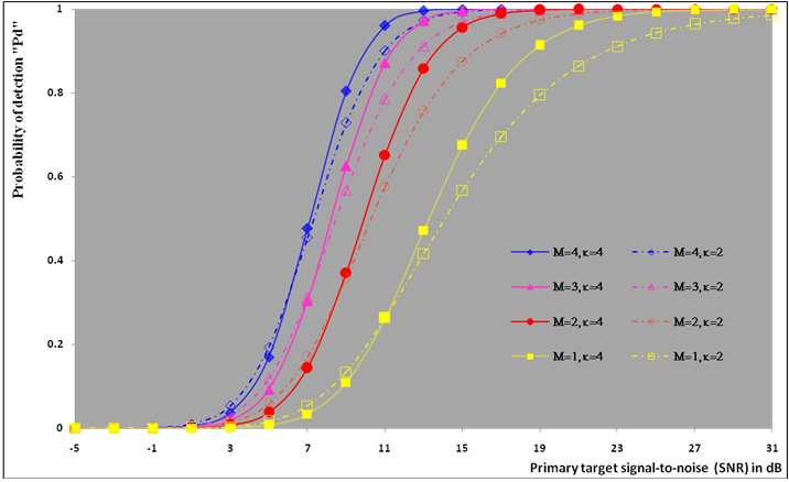
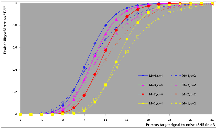
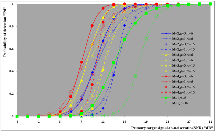
This section is devoted to the numerical evaluation of the previously-presented detection expressions of the underlined scheme for the Swerling as well as the partially-correlated χ2-models. We start our presentation by considering the case where the operating environment is ideal seeking for the highest detection performance of the DT algorithm and searching for the optimum values of the more sensitive parameters that directly affect the behavior of such type of adaptive schemes. In other words, to better understand the reaction of DT against fluctuating targets that belong to homogeneous environment, we are going to assess its performance to show the role that each parameter can play in controlling its detection characteristics. Here, it is assumed that there is a train of M pulses and a design false alarm rate of 10−6 is demanded. Theoretically, the larger a CFAR window is, the better its detection performance is (i.e., closer to the performance of the Neymann_Pearson detector), provided that the more distant cells still have the same statistics as that of the noise in the test cell. Therefore, a reference window of size N = 24 cells is adopted in processing our calculations to obtain the numerical results that are displayed throughout this manuscript. Our numerical results will be presented in several categories of curves. The first category, including Figs.(2-7), is concerned with the detection probability of the underlined scheme as a function of the signal strength for different values of its parameters. Fig.(2) depicts its behavior against fluctuating targets when the censoring threshold is held constant (τ= 10dB) and the radar receiver bases its decision on 2, 3, or 4 consecutive sweeps given that the target obeys χ2 model, with four degrees of freedom (κ=4), in its fluctuation and the correlation coefficient attains values starting from de-correlated and ending at fully-correlated passing by partially-correlated situations. For weak signal strength, the more correlated target returns give higher performance than the less correlated ones and the top case corresponds to fully-correlated (ρs=1.0) returns which belong to fluctuating targets obeying SWIII model in their fluctuation. This behavior is rapidly altered as the signal becomes strengthened. This means that there are two distinct regions in the detection performance of the DT algorithm depending on the strength of the signal returned from the target. In the first one, which is characterized by modest level of signal return, the correlation of the target returns plays an important part in improving the processor performance and the highest case corresponds to SWIII model (ρs=1.0) whilst the worst one belongs to SWIV type (ρs= 0). In other words, as the target returns become correlated, as the detection reaction enhances. This region will be denoted as SWIII-SWIV since the SWIII model gives higher detection performance than that obtained by SWIV. In the other region, the detector behavior is reversed where the correlation strength deteriorates the performance of the underlined scheme and the top detection is obtained when the target fluctuation following SWIV model while the lowest detection is achieved when the target follows SWIII type in its fluctuation. This region will be labeled as SWIV-SWIII where the SWIV model surpasses the other fluctuation case in its detection behavior. In any situation, SWIII and SWIV models embrace the partially-correlated cases with SWIII as the best one in the former region whereas SWIV gives the highest performance throughout the latter region. The degree of enhancement increases, in the first zone, or decreases, in the second zone, gradually as the correlation coefficient among the target returns varies from de-correlated to fully-correlated. Additionally, the displayed results of this figure reveal, in an explicit form, that the pulse integration improves the CFAR performance as it combats the deep fades and the loss of the signal. Moreover, as M increases, the point of transition from the SWIII-SWIV zone to SWIV-SWIII one is shifted towards lower signal strengths. Fig.(3) illustrates the same thing as the previous scene taking into account that all the parameter values are held unchanged except that the degrees of freedom is varied from 4 to 2 in order to know to what extent the parameter κ can impact the behavior of the adaptive procedure. The family of curves of this plot behaves as the previous ones with some minor degradation and negligible values for the signal strength at which the change from the former region to the other region occurs. Fig.(4) describes the detection probability, as a function of the signal power, when the primary target fluctuates in accordance with χ2 model with four degrees of freedom (κ=4) and for several values for the correlation strength among the target returns given that the radar receiver based its decision on integrating 2 and 4 consecutive pulses. For the purpose of comparison, the single sweep case is included among the curves of this plot to illustrate to what extent the technique of pulse integration can ameliorate the processor performance. In addition, the excision threshold is updated to become τ=17.5dB in order to take an idea about the influence of this threshold on the behavior of the DT-CFAR scheme in detecting the searched target. An insight examination of the behavior of the curves of this scene reveals that they follow the same variation as those of Fig.(2) with a negligible minor deterioration indicating that the trimming threshold has an insignificant impact on the processor performance as it increases from 10dB to 17.5dB taking into account that the operating environment is free of any interferers. Additionally, it is observed that the mono-pulse curve is the worst one among the candidates of this plot signifying that the integration of successive pulses enforce the returned signal and consequently enhance the processor performance.It is of importance to combine the situations of κ=4 and κ=2 on the same figure to simultaneously compare the reaction of the tested algorithm against that target the fluctuation of which follows χ2 statistics with different degrees of freedom. This is the object of Fig.(5) which shows the same characteristics as the previous figures with different parameter values. In this plot, Pd is drawn against SNR for several values of the correlation coefficient "ρs" when M=3 given that the searched target fluctuates following χ2-model with κ=2 & 4 and the excision threshold is augmented to become 25dB. To visualize the gain that can be achieved through the integration of pulses, the single-sweep characteristic is merged with the curves of this scene. The careful examination of the elements of this figure indicates that they follow the same behavior as their corresponding ones in the previous plots with minor variations. In these circumstances, the first region is characterized by SWI-SWIII-SWII-SWIV formulation which means that the SWI model has the highest performance whilst the SWIV fluctuation model presents the worst reaction in this situation of operation. As the returned signal becomes stronger, the reverse of this sequence is clearly observed. For the mono-pulse operation, the figure shows that the processor gives its highest performance when the primary target fluctuates in accordance with χ2-distribution with κ=2 when operating in the former region whereas this behavior is reversed in the other region.The next plot in the detection group of figures is devoted only to the Swerling cases where the fluctuating target returns are de-correlated (ρs=0) and the fluctuation obeys χ2-distribution with κ=2 & 4. Under these conditions of operation, Fig.(6) displays the detection characteristics of DT(17.5) processor for integrated pulses of 4, 3, and 2 along with the single-pulse case. The curves of this scene follow the same manner in their variations as the previous ones confirming the previous concluded remarks that SWII model exhibits better performance for weak signal whilst the detection reaction of SWIV model surpasses that of SWII model when the returned signal becomes stronger. Additionally, the gap between the two performances decreases as the number of integrated pulses increases. Fig.(7) repeats the same thing as that presented in Fig.(6) except that the target returns are assumed to be fully-correlated (ρs=1). In other words, this figure is interested in presenting the processor detection reaction against SWI and SWIII models. In this case, the first zone is privileged by SWI model which exhibits higher performance than the SWIII model. The second zone, on the other hand, is distinguished by SWIII model the detection performance of which exceeds that of SWI model. The mono-pulse processor performances, for κ=2 & 4, behave exactly like the corresponding ones in Fig.(6) with some degradation. Additionally, the difference between the two performances, for the same number of integrated pulses, rests approximately constant independent upon the number of integrated consecutive sweeps. 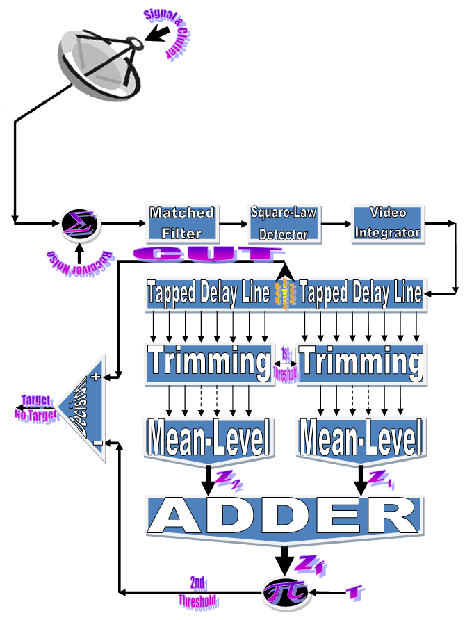 | Figure (1). M-sweeps architecture of double-threshold adaptive algorithm |
 | Figure (2). Ideal M-sweeps detection performance of DT(10.0)-CFAR procedure for partially-correlated  targets when N=24, targets when N=24,  and Pfa=10-6 and Pfa=10-6 |
 | Figure (3). Ideal M-sweeps detection performance of DT(10.0)-CFAR procedure for partially-correlated  targets when N=24, targets when N=24,  and Pfa=10-6 and Pfa=10-6 |
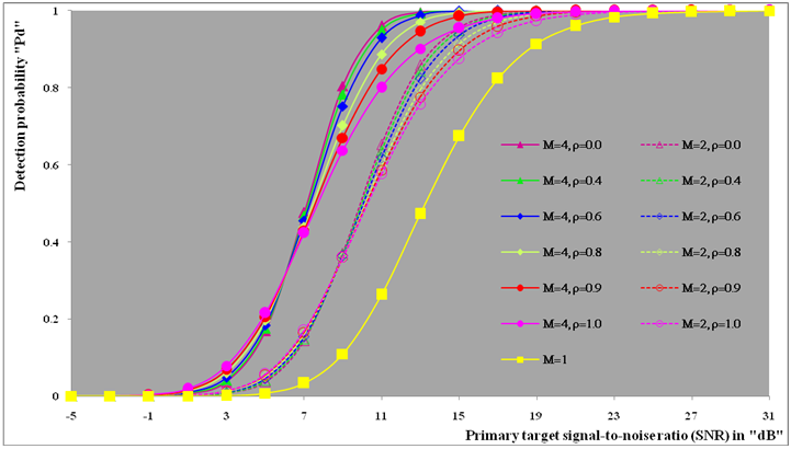 | Figure (4). Ideal M-sweeps detection performance of DT(17.5)-CFAR procedure for partially-correlated  targets when N=24, targets when N=24,  and Pfa=10-6 and Pfa=10-6 |
 | Figure (5). Ideal M-sweeps detection performance of DT(25)-CFAR procedure for partially-correlated  targets when N=24, M=3, targets when N=24, M=3,  and Pfa=10-6 and Pfa=10-6 |
 | Figure (6). Ideal M-sweeps detection performance of DT(17.5)-CFAR procedure for partially-correlated  targets when N=24, targets when N=24,  and Pfa=10-6 and Pfa=10-6 |
 | Figure (7). Ideal M-sweeps detection performance of DT(17.5)-CFAR procedure for partially-correlated  targets when N=24, targets when N=24,  and Pfa=10-6 and Pfa=10-6 |
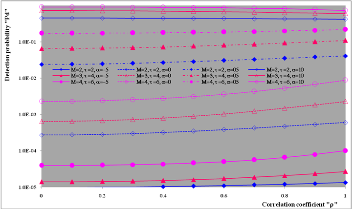
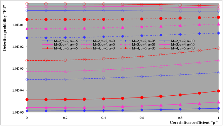
The second category of our numerical results, that are associated with homogeneous environments, includes Fig.(8) which measures the capability of the processor to detect fluctuating targets in ideal reference channels. In the radar terminology, the characteristics of this figure are known as receiver operating characteristics (ROC's). They describe the detection probability against the false alarm rate for a signal strength of 5dB when the radar receiver integrates 2, 3, and 4 consecutive sweeps given that the primary target follows χ2-distribution with κ=4 in its fluctuation and its returns are either de-correlated or fully-correlated. The optimum detector is included among the contents of this figure for the purposes of comparison. The ROC's of the DT scheme, with numerous values for its censoring threshold, along with those representing the optimum system are traced keeping into account that the operating conditions are held unchanged in the two cases for the comparison to be explicitly clear. A label (DT(4), SWIII, 3) on a specified curve means that it is associated with the DT processor the excision threshold of which is 4dB, the primary target complies SWIII in its fluctuation, and the process of detection is carried out through the integration of 3 successive pulses. On the other hand, a label like (opt, SWIII, 3) on a given curve symbolizes the same things for the optimum detector. Since the excision threshold has a minimum value below which no one of the reference samples is capable to survive after crossing it, the values 2, 4, and 6dB for this threshold are selected to obtain the results of the current figure where they represent the minimum values of the trimming threshold (τmin) for M=2, 3, and 4, respectively. The illustrated results of this plot indicate that its family of curves behaves like those of the detection performance from the strength of correlation point of view. For low rate of false alarm, SWIII fluctuation model presents higher detection reaction than SWIV model. As the false alarm rate augments, this behavior is altered. The inflection point moves towards lower probability of false alarm as M increases and the performance of the optimum processor is always proceeding that of the DT scheme the trimming threshold of which doesn't allow any abnormal sample to penetrate it.The last category in this group of curves is associated with the variation of the processor characteristics as a function of the strength of correlation among the target returns including the partially-correlated along with the two boundaries which represent the uncorrelated and the totally correlated. The scope of the first plot in this category is to compute the required signal strength, to achieve a specified level of detection, as a function of the correlation coefficient "ρs" for several values of integrated pulses when the fluctuation of the primary target complies χ2-distribution with κ=2 & 4. The obtained results are illustrated in Fig.(9). The investigation of this figure demonstrates that there is a negligible increment in the SNR, required to attain a detection level of 90%, as the correlation among the target returns enforces and this increment becomes noticeable as these returns being highly correlated. For κ=4, the processor achieves the request level of detection with lower signal strength than the case where the degrees of freedom is 2, as predicted. Additionally, the rate of increasing near the upper limit of ρs, when the target fluctuates with κ=2, is higher than that in the case where the target fluctuation follows χ2-distribution with κ=4. Furthermore, the DT scheme with τ=10dB acquires less SNR in attaining 90% detection level in comparison with that the excision threshold of which is 2dB, given that the number of integrated pulses is 2. The same thing occurs for M=3 where τ=10dB for the trimming threshold of DT algorithm realizes the pre-assigned level of detection with smaller signal strength than that enquired by DT(4) scheme, given that the case of fluctuation remains unchanged. However, there is approximately no difference between the SNR's required by DT(6) and DT(10) procedures to arrive at the same previously mentioned level of detection in the case of M=4. The behavior of this family of curves demonstrates that SWII model, in the case of κ=2, and SWIV model, in the case of κ=4, accomplish higher detection performance than their corresponding models at the upper limit of correlation and for the same degrees of freedom. The last scene in this category describes the processor detection performance as a function of the correlation strength among the target returns for some values of SNR and integrated pulses. Fig.(10) displays the results of this group for a DT scheme the censoring threshold of which is allowed to vary from 2dB to 6dB with a step of 2dB and its signal strength takes distinct levels starting from -5dB up to 10dB with an increment of 5dB, knowing that the primary target complies χ2-distribution with κ=4 in its fluctuation. For lower values of the censoring threshold, the detection reaction of the tested algorithm improves as the correlation among the target returns increases given that the signal strength is weak. As the SNR increases, the rate of improvement decreases gradually and tends to be negligible as the target returns become strengthened. For τ = 6dB, on the other hand, the processor detection behavior varies in the same manner as its corresponding one in lower τ values except that it tends to decrease as ρs increases for higher values of SNR. Now, let us turn our attention to the application of the DT algorithm for target detection under severe interference. We will present our numerical results in several categories of curves. The first category is concerned with the processor detection performance in the presence of spurious targets for different operating conditions. This category includes Figs.(11-12). The first scene in this group, Fig.(11), plots the detection probability against SNR for M=2, 3, and 4 along with the single sweep case when there are 5 extraneous targets of the same fluctuating model as that of the tested target (ρi=ρs) and the two target types, primary and interfering, return signals of similar strength (INR=SNR). The excision threshold of the DT scheme is chosen to have 6 and 16dB values to show its role in improving the detector behavior against outlying targets when their number becomes intense. Additionally, the primary and the secondary interfering targets are assumed to be fluctuating in accordance with χ2-distribution with 4 degrees of freedom and the returns of each target are either de-correlated (SWIV model) or fully-correlated (SWIII model). An insight into the variation of the curves of this figure demonstrates that DT(6) algorithm surpasses, in its detection reaction, DT(16) processor in any situation of operation even in mono-pulse case. In other words, the processor performance in the case of DT with τ=16dB is degraded in comparison with that of DT with τ=6dB. This behavior is predicated because as the censoring threshold increases, the likelihood of contaminated reference channels with spurious target returns increases and this in turn results in raising the detection threshold and consequently the processor performance becomes worsen. On the other hand, the detection probability follows the same behavior as in the case of ideal environment given that the trimming threshold is kept constant. The last plot in this category, Fig.(12), is associated with the detection reaction of DT, for several values of the trimming threshold, against multitarget environment when the tested as well as the undesired targets fluctuate according to four degrees of freedom χ2-process and their returns present null or fully correlation among them keeping into mind that two successive pulses are combined to carry out the decision process. It is clear that as τ increases, the target returned signal must be strengthened for the detector to become capable to decide its presence. For mono-pulse case, on the other hand, increasing the censoring threshold makes the DT scheme unable to detect the searched target in contaminated reference channel especially if the number of infected samples augments. The results outlined in this category demonstrate the role that the censoring threshold can play in the reaction of the double-threshold detector against an interference saturated environment and consequently, the good selection of which is our scope in this research for the detector performance achieves its highest allowable reaction when the operating environment is of target multiplicity.There is another type of characteristics that measure the capability of the processor to detect targets in contaminated reference channels. It is of primary concern to examine the effects of interfering targets on the ability of the underlined scheme to maintain the required rate of false alarm fixed, where the task of keeping a near-constant probability of false alarm represents the fundamental requirement in radar detection problems. We present some numerical results that demonstrate the performance of DT-CFAR detector when the sample set has some of its cells that are contaminated with interfering target returns of equal strength. The associated figures of this category of plots comprises Figs.(13-14). The first candidate of this family illustrates the false alarm rate as a function of the strength of interference for several values of integrated pulses when the spurious targets exhibit, in their fluctuation, χ2-statistics with 4 degrees of freedom and their returns have zero or unity correlation coefficient given that the excision threshold is held constant at 6dB or 16dB and the designed rate of false alarm is 10-6. As shown in Fig.(13), the rate of false alarm is approximately constant when τ=6dB and the correlation among the interferer returns has approximately no impact on the false alarm rate performance of the tested scheme. Additionally, the processor performance enhances as the number of integrated pulses increases and as the target returns become strengthened. This behavior is logic since lowering the trimming threshold decreases the chance for the interferer sample to escape from the trimming threshold and therefore prevents it from participating in establishing the detection threshold which becomes representing the homogeneous case and consequently the false alarm rate tends to its designed value. As the excision threshold increases, the appearance of what is known as an ineffectiveness zone is noticed. The ineffectiveness zone is the range below the censoring threshold in which interferers are not eliminated and therefore influence the setting of the detection threshold. This zone is characterized by decreasing the rate of false alarm whenever the interfering returns are modestly strengthened. As the strength of the outlier returns becomes stronger, the false alarm rate changes its slope towards its design value and holds constant when the interferer returns are highly strengthened. The examination of the variation of this specified zone indicates that the correlation among the extraneous target returns as well as the post-detection integration enhance the false alarm rate of DT processor. Additionally, the gap between the minimum attainable level of false alarm and the required rate decreases as M increases, given that the correlation characteristics of the interferer returns are held constant. Moreover, the size of this gap is minimum in fully-correlated case whilst it becomes maximum in the case of de-correlated as long as the other parameter values are kept unchanged. It is of importance to note that the size of this gap tends to be vanished for lower values of the trimming threshold as Fig.(13) demonstrates. Fig.(14), on the other hand, illustrates the same thing as that presented in the previous figure on the exception that the censoring threshold is allowed to have larger values to show its role in controlling the false alarm rate of DT procedure. Three non-coherently integrated pulses (M=3), when the target returns have SWIII or SWIV fluctuation model, are taken into account in tracing this plot. For low values of the censoring threshold τ, the false alarm probability remains approximately constant with small deviations from the design value, given that the extraneous target returns are weakly strengthened, and these deviations are rapidly decreased, as either the interferer's strength or the censoring threshold increases, till a specified level of interference beyond which the false alarm probability increases towards its design value. The interference level at which the slope of a given curve is altered increases as the excision threshold increases. This behavior is physically logic since increasing τ means increasing the signal strength of the reference cell for the trimming process to be able to prevent it from participating in implementation of the detection threshold. This processing is continued till an interference level at which all the interfering cells are rejected from the cell-averaging operation and consequently, the false alarm rate returns to its design value at that level of interference. In the limit, as the censoring threshold tends to infinity, τ → ∞, Pfa decreases rapidly with INR and the interference level that exchanges the slope of the curve tends to be infinity owing to the surviving of all the interferers which raises the detection threshold and consequently decreases the false alarm probability intolerably. For the same censoring threshold, the SWIII model for the extraneous target fluctuation gives better false alarm rate performance than the case of SWIV fluctuation model. Additionally, each group of curves for SWIII or SWIV model follows the same slope as the trimming threshold varies where SWIV model presents larger slope than that followed by SWIII model. In any situation, the slope of decreasing increases as τ increases, as shown in the figure. Moreover, the point of changing the slope from negative to positive is shifted towards heavier interference as the excision threshold augments and this is common irrespective to the spurious target fluctuation model. In other words, the false alarm rate performance improves; i. e. more nearer to the required value, as the interferer returns become strongly correlated. An another important category of curves is that concerned with the detection performance as a function of the strength of correlation among the target returns, for minimum allowable values of the trimming threshold and several values of integrated pulses, in the presence of 5 contaminated samples among the elements of the reference set when the primary as well as the secondary interfering targets fluctuate obeying χ2-distribution with 4 degrees of freedom. Fig.(15) depicts these characteristics for multi-values of signal strength for both kinds of targets (INR=SNR) taking into account that their returns have the same strength of correlation (ρi=ρs). Since the post-detection integration makes the signal strengthened and the rate of strengthened increases as M increases, the minimum τ values are 2, 4, and 6 for M=2, 3, and 4, respectively. The minimum value in this text means that value below which there is no detection owing to the intolerable value of the threshold. These values are the optimum ones for which the DT scheme exhibits its optimum detection performance as Fig.(15) demonstrates. As we have previously stated, the detection probability improves as the correlation among the target returns increases when the intensity of the received signal is weak and this is explicitly evident from the displayed results. For strong signal returns, on the other hand, the processor performance returns to its natural case where the correlation degrades it and the degree of degradation increases as the signal returns become strongly correlated. Also, the processor performance enhances as M increases under any situation of operation. The next plot in this category is devoted to present, in a clear manner, the effect of τ on the behavior of the DT algorithm in deciding the presence of the searched target in contaminated reference channel. Fig.(16) clarifies the required SNR to make the underlined processor able to decide the presence of primary fluctuating target with a detection level of 90% on the condition that the estimation set has 5 cells, among its elements, infected by outlier returns of the same strength as well as correlation as the primary target. As shown, the needed SNR is approximately constant till τ=14dB beyond which it increases in a nearly linear manner with increasing τ. It is of importance to note that the minimum value of τ, for M=4, is 6dB. Under the same set of operating conditions, the fluctuation model follows 4 degrees of freedom χ2-statistics requires less SNR in comparison with that of 2 degrees of freedom χ2-distribution and the fluctuation of fully-correlated 4 degrees of freedom is coincided with the de-correlated 2 degrees of freedom when M=2. In addition, as M increases, the difference between the SNR needed for null-correlated χ2-statistics with 4 & 2 degrees of freedom decreases whilst it remains approximately unchanged for unity-correlated χ2-statistics with 4 & 2 degrees of freedom, at the same level of the censoring threshold. In the last category of curves, we are interested in showing the variation of the processor detection performance with the number of spurious target returns that may exist amongst the candidates of estimation channels. The elements of this family of curves are two figures, Figs.(17-18). Each one of this family illustrates the variation of the detection probability as a function of the number of extraneous targets, parametric in the degrees of freedom and the number of integrated pulses. Fig.(17) shows the DT detection reaction against the density of interferers that may exist in the operating environment for several values of the excision threshold in the case where the target under test along with the spurious ones fluctuate according to χ2-model with 4 degrees of freedom and their returns are either de-correlated or fully-correlated when the CFAR circuit collects its data from two consecutive sweeps to tackle its detection. Both types of targets generate the same signal strength (SNR=INR=10dB) at the decision circuit. For the purpose of comparison, the single-sweep results are incorporated amongst the elements of this plot. The examination of this drawn reveals that the DT scheme has immunity to the presence of outliers, even if the number of contaminated samples excesses half the size of the reference set when its censoring threshold is chosen to be low. This behavior is general even for mono-pulse operation. This immunity is due to excising the outlying returns and prohibiting them from the construction of the detection threshold. As the trimming threshold increases, the processor tends to deprive this important property; especially when the number of extraneous targets is large. In the limit, the DT algorithm tends to behave like the conventional CA scheme in tackling the operation of target multiplicity. In other words, as τ → ∞, the underlined detector becomes un-capable in deciding, with high probability, the presence of the searched target in the case where the operating environment contains outliers other than the target under test. As a final remark about Fig.(17) is that there are two groups of curves: one representing the single-sweep case and the other denotes the double-sweep case with special gain owing to post-detection integration. Each group starts from the same point which belongs to homogeneous situation (R=0) and remains unchanged, when τ is low, or degrades as R increases, when τ becomes large. The next plot in this category is interested in showing the impact of the degrees of freedom on multi-target performance of the DT detector. Fig.(18) traces the probability of detection as a function of the number of fluctuating interferers when the radar receiver seeks for the desired fluctuating target given that the two types of targets excite the same signal strength at the input of the CFAR circuit the excision threshold of which is selected to be 16dB. The candidates of this trace are parametric in M, ρ, and κ. An insight into the displayed results indicates that there are four families of curves: one for each value of M. For small values of outliers, the fluctuating targets with 4 degrees of freedom give better performance than those fluctuating with 2 degrees of freedom and the de-correlated case exceeds in its detection probability the full-correlated case. As the number of interferers increases, the behavior is completely reversed making SWI model in the top and SWIV model in the bottom of this family. This behavior is common for any number of integrated pulses taking into account that the point of altering is shifted towards upper number of spurious targets as M increases. In the single sweep case, the fluctuation with 2 degrees of freedom surpasses in its detection that obtained from fluctuation with 4 degrees of freedom since the signal strength is modest (SNR=INR=10dB). It is of interest to note that the detector performance improves as either the correlation among the fluctuating target returns weakens, as the number of post-detection integrated pulses increases, or as the degrees of freedom of the χ2-distribution increases given that the signal strength is strong and the remaining parameters are held unchanged.
5. Conclusions
This paper has addressed the problem of CFAR detectors designed to operate in an interference saturated environment. In such an environment the performance of the conventional cell-averaging detectors can be drastically degraded, owing to the inevitable influence of the outlying samples on the sample average that is used for implementation of the detection threshold. The analytical results have been associated with an application in which the DT detector is supplemented by a post-detection integrator. The purpose of the integrator is to diminish the effect of strong random interfering signals while enhancing the detection probability of a periodic sequence of pulses. The numerical results should provide an important insight into the effect of the system’s parameters on its performance.We have given a detailed derivation of the detection performance of the DT-CFAR processor in multi-target situations. This type of radar detectors combats the effect of variations in the noise level and interferences by adapting the detection threshold to the sample average and by neutralizing the effect of strong interfering signals by discarding them prior to the cell averaging operation. Even if not all interferers are removed, the elimination of the strongest ones among them and therefore the most damaging to processor performance, is assured. 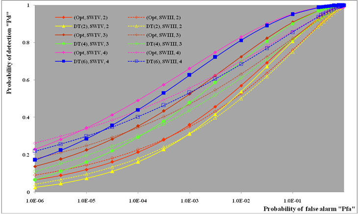 | Figure (8). Ideal M-sweeps Receiver Operating Characteristics (ROC's) of  scheme for partially-correlated scheme for partially-correlated  targets when N=24, targets when N=24,  |
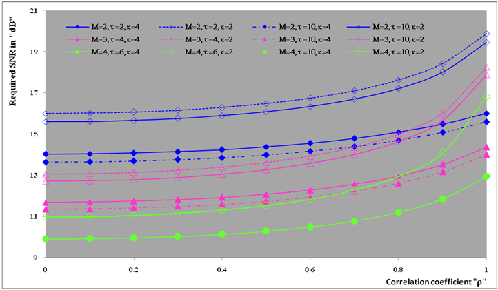 | Figure (9). Ideal M-sweeps required SNR to attain a detection level of 90% of  scheme for partially-correlated scheme for partially-correlated  targets when N=24, targets when N=24,  and Pfa=10-6 and Pfa=10-6 |
 | Figure (10). Ideal M-sweeps detection performance of  scheme for partially-correlated scheme for partially-correlated  targets when N=24, targets when N=24,  and Pfa=10-6 and Pfa=10-6 |
 | Figure (11). Multitarget M-sweeps detection performance of  scheme for partially-correlated scheme for partially-correlated  targets when N=24, R=5, targets when N=24, R=5,  INR=SNR, and Pfa=10-6 INR=SNR, and Pfa=10-6 |
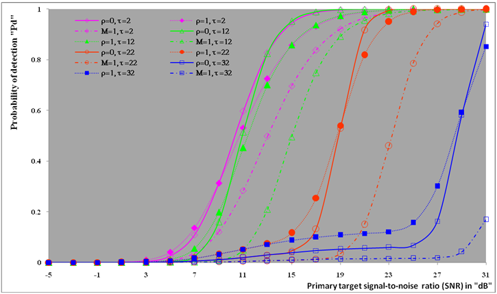 | Figure (12). Multitarget M-sweeps detection performance of  procedure for partially-correlated procedure for partially-correlated  targets when N=24, M=2, targets when N=24, M=2,   and Pfa=10-6 and Pfa=10-6 |
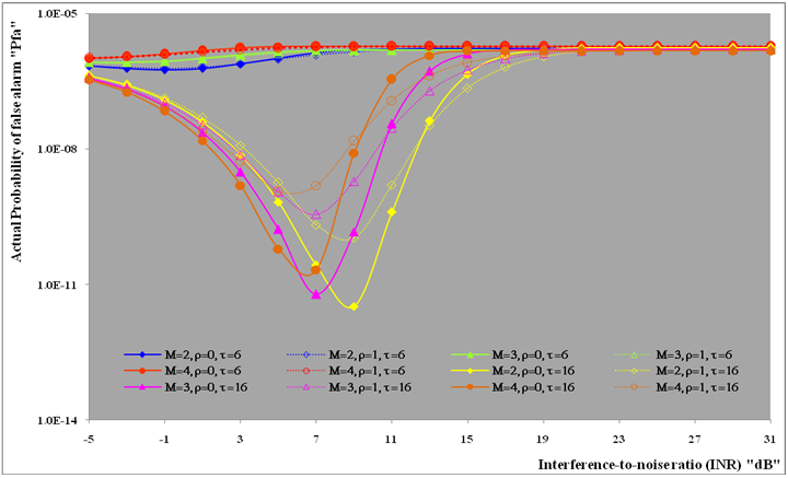 | Figure (13). Multitarget M-sweeps false alarm rate performance of  scheme for partially-correlated scheme for partially-correlated  targets when N=24, targets when N=24,  R=5, and design Pfa=10-6 R=5, and design Pfa=10-6 |
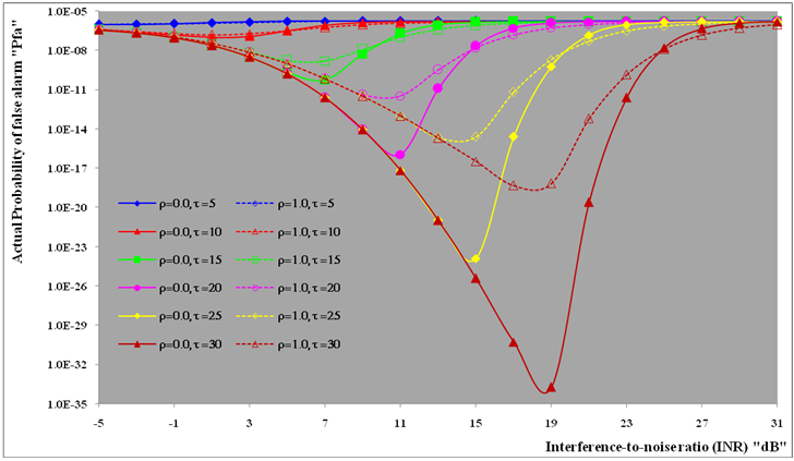 | Figure (14). Multitarget M-sweeps false alarm rate performance of  scheme for partially-correlated scheme for partially-correlated  targets when N=24, targets when N=24,  M=3, R=5, and design Pfa=10-6 M=3, R=5, and design Pfa=10-6 |
 | Figure (15). Multitarget M-sweeps detection performance of  scheme for partially-correlated scheme for partially-correlated  targets when N=24, R=5, targets when N=24, R=5,  and Pfa=10-6 and Pfa=10-6 |
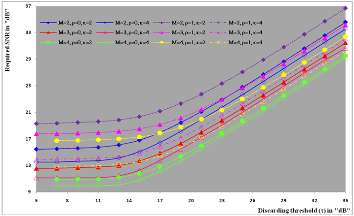 | Figure (16). Multitarget M-sweeps required SNR, to attain a detection level of 90%, of  scheme for partially correlated scheme for partially correlated  targets when N=24, targets when N=24,  R=5, and Pfa=10-6 R=5, and Pfa=10-6 |
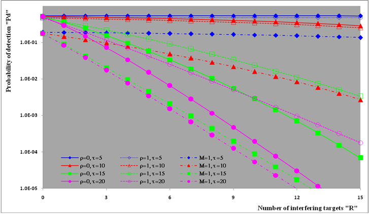 | Figure (17). Multitarget M-sweeps detection performance of  scheme for partially-correlated scheme for partially-correlated  targets when N=24, M=2, targets when N=24, M=2,  INR=SNR=10dB, and Pfa=10-6 INR=SNR=10dB, and Pfa=10-6 |
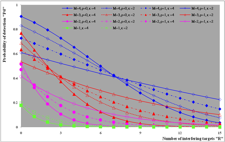 | Figure (18). Multitarget M-sweeps detection performance of  scheme for partially-correlated scheme for partially-correlated  targets when N=24, targets when N=24,  INR=SNR=10dB, and Pfa=10-6 INR=SNR=10dB, and Pfa=10-6 |
The determination of the DT parameters will be outlined. For this detector to be effective, τ should be set as low as possible for preventing any sample, that is not belong to noise, from participating in the construction of the detection threshold; but if the input signal is infected by a wideband jamming signal, a low τ can result in trimming most of the noise samples, and therefore cause a drastic degradation in performance. On the other hand, if the excision threshold is set too high, an ineffectiveness zone, the width of which is the ratio between the censoring threshold and the mean value of the actual noise level, is created. The samples in this zone which originate from various spurious transmissions are not trimmed.
References
| [1] | Win-Qin Wang (2013) “Radar systems: Technology, Principles, and Applications”, Nova Science Publishers, Inc., 2013. |
| [2] | Conte, E., Longo, M. & Lops, M. (1989), “Analysis of the excision CFAR detector in multiple target situations”, In Proceedings of the 1989 IEICE International radar symposium, 1989, pp. 565-571. |
| [3] | El Mashade, M. B. (1997) “Performance analysis of the excision CFAR detection techniques with contaminated reference channels”, Signal Processing “ELSEVIER”, Vol. 60, (July 1997), pp. 213-234. |
| [4] | Dong-Seong Han (2000), "Detection performance of CFAR detectors based on order statistics for partially correlated chi-square targets", IEEE Transactions on Aerospace and Electronic Systems, Vol. 36, No. 4, (Oct. 2000), pp. 1423 – 1429. |
| [5] | El Mashade, M. B. (2001), "Postdetection integration analysis of the excision CFAR radar target detection technique in homogeneous and nonhomogeneous environments", Signal Processing “ELSEVIER”, Vol. 81 (2001), pp.2267–2284. |
| [6] | El Mashade, M. B. (2002), “Target Multiplicity Performance analysis of radar CFAR detection techniques for partially correlated chi-square targets”, Int. J. Electron. Commun. (AEŰ), Vol.56, No.2, (April 2002), pp. 84-98. |
| [7] | El Mashade, M. B. (2006), “Performance Evaluation of the Double-Threshold CFAR Detector in Multiple-Target Situations”, Journal of Electronics (China), Vol.23, No.2, (March 2006), pp. 204-210. |
| [8] | El Mashade, M. B. (2008), “Performance Improvement of Adaptive Detection of Radar Target in an Interference Saturated Environment”, Progress In Electromagnetics Research M, Vol.2, pp. 57-92, 2008. |
| [9] | El Mashade, M. B. (2011), M-correlated sweeps performance analysis of adaptive detection of radar targets in interference- saturated environments", Ann. Telecommun. (2011), Vol. 66, pp. 617–634. |
| [10] | El Mashade, M. B. (2011), “Analysis of adaptive detection of moderately fluctuating radar targets in target multiplicity environments”, Journal of the Franklin Institute, Vol. 348, No. 6, (2011), pp. 941–972. |
| [11] | El Mashade, M. B. (2013), "Analytical Performance Evaluation of Adaptive Detection of Fluctuating Radar Targets", Radioelectronics and Communications Systems, 2013, Vol. 56, No. 7, pp. 321–334. |
| [12] | G. Cui, A. De Maio, and M. Piezzo, (2013), “Performance prediction of the incoherent radar detector for correlated generalized swerling-chi fluctuating targets”, IEEE Transactions on Aerospace and Electronic Systems, Vol. 49, No. 1, pp. 356–368, January 2013. |
| [13] | El Mashade, M. B. (2013), "Multiple-target analysis of adaptive detection of partially correlated χ2 targets", Int. J. Space Science and Engineering, Vol. 1, No. 2, 2013, pp.142-176. |
| [14] | El Mashade, M. B. (2013), "Post detection Integration Analysis of Adaptive Detection of Partially-Correlated χ2 Targets in The Presence of Interferers", Majlesi Journal of Electrical Engineering, Vol. 7, No. 3, September 2013, pp. 43-58. |
| [15] | El Mashade, M. B. (2014), "Partially-Correlated χ2 Targets Detection Analysis of GTM-Adaptive Processor in the Presence of Outliers", I.J. Image, Graphics and Signal Processing, 2014, 12, pp.70-90. |

 Abstract
 Reference
 Full-Text PDF
 Full-text HTML