Salah H Abid , Ali S Rasheed
Al-Mustansirya University – Education College-Mathematics Department
Correspondence to: Salah H Abid , Al-Mustansirya University – Education College-Mathematics Department.
| Email: |  |
Copyright © 2012 Scientific & Academic Publishing. All Rights Reserved.
Abstract
Spectral estimates depend for their specification on a truncation point and Lag window. New Lag window is suggested to estimate the spectral density function of Low order autoregressive processes, AR(1) and AR(2). This New Lag window based on a family of densities suggested by Johnson, Tietjen and Beckman (JTB). A comparison among a wide range of Lag windows is presented based upon empirical experiments. The New Lag window was the best of all other Lag windows in most of cases.
Keywords:
Lag Window, Spectral Density Estimation, AR Processes
Cite this paper: Salah H Abid , Ali S Rasheed , New Lag Window for Spectrum Estimation of Low Order AR Processes, American Journal of Signal Processing, Vol. 3 No. 4, 2013, pp. 85-101. doi: 10.5923/j.ajsp.20130304.01.
1. Introduction
Let  be a real valued, weakly stationary, discrete stochastic process (time series) with zero mean and autocorrelation function
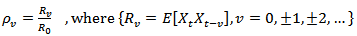 | (1) |
If one has series of size  , then the consistent form to estimate the spectral density function is[10]
 | (2) |
Where  is the truncation point
  and
and  where
where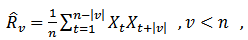 | (3) |
And  is the lag window.To get a good estimate of
  , one must select an appropriate value of
  and an appropriate function of
  .The above approach is shown to be a special case of smoothing a sample spectrum estimator by giving decreasing weight to the autocovariances as the lag increases. The weighting function is known as the lag window (kernel) and leads to a smoothed spectral estimator.NEAVE 1972[8] explained that Spectrum estimates depend for their specification on a truncation point and a "covariance averaging kernel" or "lag window," which is derived from a "lag window generator." A comparison of such generators is presented, based upon their negated derivatives, which are shown to be the approximate weightings in a particular type of representation of the spectrum estimate. It is clearly shown why the well-known generators of Parzen and Tukey are superior to most (but not all) of their rivals. Neave stated that “These still have weaknesses, however, and the article concludes with a suggestion how these may be overcome”.In 1978, Harris[4] paper includes a comprehensive catalog of data windows along with their significant performance parameters from which the different windows can be compared. Also, an example demonstrates the use and value of windows to resolve closely spaced harmonic signals characterized by large differences in amplitude.In 1981 Nuttall[9] studied some windows with very good sidelobes behavior some windows with very good sidelobes behavior which means in terms of bias due to nearby sidelobes and bias due to distant sidelobes.Hannover in 2002[5] gave a practical overview about the estimation of power spectral densities using the discrete Fourier transform and the fast Fourier transform. And emphasized on the relationship between estimates of power spectra and power spectral densities which is given by the effective noise bandwidth (ENBW). Included is a detailed list of common and useful window functions, among them the often neglected flat-top windows. Special highlights are a procedure to test new programs, a table of comprehensive graphs for each window and the introduction of a whole family of new flat-top windows.In 2009 Hongwei[6] used multi-instrument to evaluation of various window functions which are analyze the window function WAV file with no window function and analyze a unit DC signal with the window function to be evaluated, and then evaluate of window function parametersIn 2010 Albrecht[1] explained tailoring of minimum sidelobes cosine-sum windows for high-resolution measurements.In 2012 Abdus Samad[3] proposed, a novel window function. Such windows, including the Hanning, Hamming, Blackman and Gaussian windows are useful in spectral analysis applications where a sampled signal is multiplied by such a window, usually followed by a discrete Fourier transform (DFT) in order to control spectral roll-off, generally at the expense of spectral resolution.A general feature of lag windows is that they give less weight to
  as the modulus of
  increases. Several different criteria have been proposed in the literature for evaluating different lag window spectral estimators. One of the more useful is the mean square error which is dependent on here.There are a lot of Lag windows, suggested by authors, also a lot of studies to compare among them numerically and analytically. Table (1) contains a wide range of Lag windows.
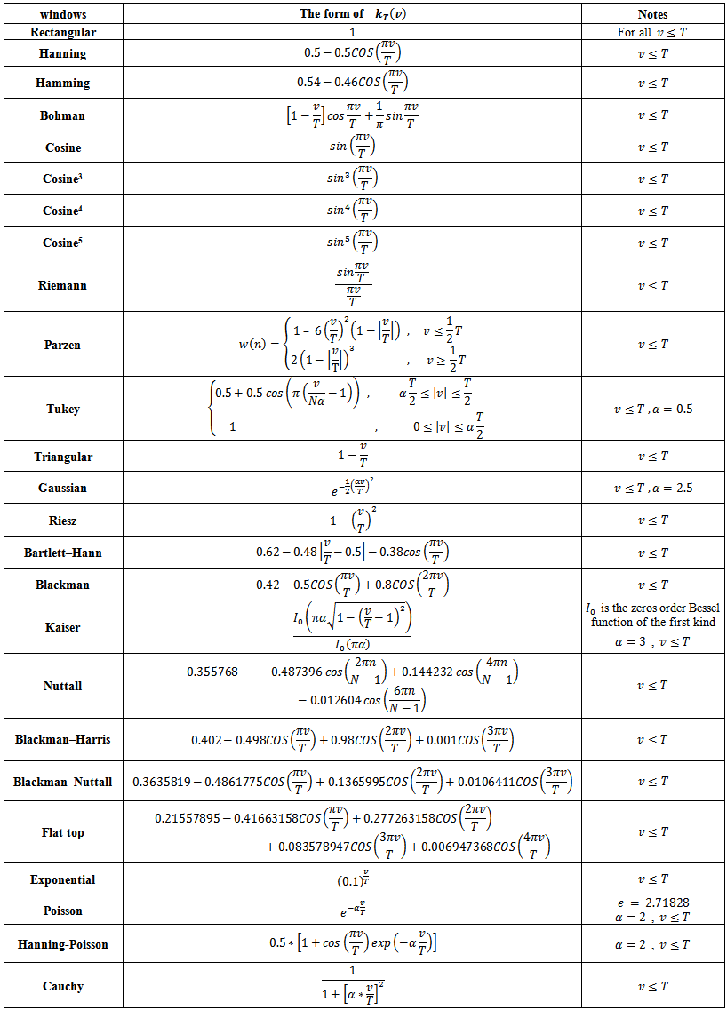 | Table (1). Lag windows |
In this work, we will suggest a new Lag window and then compare the results, empirically, of the spectral density functions constructed by the suggested lag window and by the other lag windows stated in table(1) for AR(1) and AR(2) processes, with a wide range of cases and series sizes. The comparison will be based on the mean square error criterion as mentioned above.
2. New Lag Window
In 1980, Johnson, Tietjen and Beckman (JTB)[7], Suggested a new family of probability distributions with the following density, | (4) |
Where 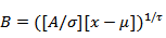 and
and 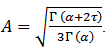 The parameters
  and
and  location and scale parameters, respectively;
  and
and  are shape parameters. This distribution is unimodal and symmetric about
  . A random variable
  with density (4) has mean
  and variance
  Moreover if
  and
and  then,
then,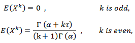 In particular, the coefficient of kurtosis
  is,
is,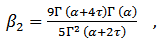 | (5) |
These moment derivations can be performed by using the moment-generating function of  ,
,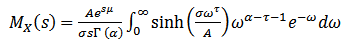 | (6) |
Several densities for which  are plotted in Figure (1). Each of these distributions has zero mean, unit variance, zero skewness, and kurtosis equal to three. A considerable degree of shape differences is observed.
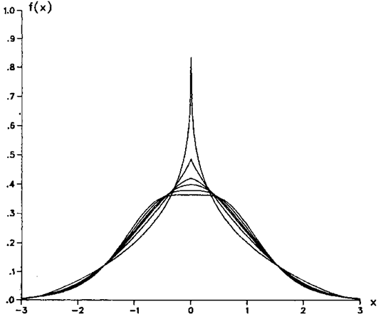 | Figure (1). illustrated Six Densities Having   |
Figure (2) provides additional density plots for 
 , and
, and  varying as indicated. These densities look very similar to those in Figure (2). Here, however, the corresponding kurtosis values are given, as follows:
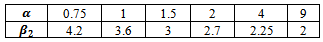 By comparing the two figures in the range
  , it is clear that kurtosis is a measure of tail behavior.
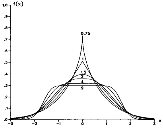 | Figure (2). illustrated Six Densities Having   |
There are two reasons to suggest this family of densities as Lag window, the first one is the high flexibility since it is contains four parameters. The second reason is that in a lot of cases, the shape of JTB family of densities is close to the ideal window shape. Since the JTB Family satisfy 
 and
and  and it is continuous for all
  , then one can use it as Lag window function.
3. Empirical Aspect
A simulation Experiment was conducted to satisfy our Research goal, by using Matlab software according to the following assumptions,1) Generate AR(1) process,  , and AR(2),
  , With the following values
  and
and  ,2) The series sizes
  3) The Run size value was
  .4) The truncation point value
  was calculated according to the closing window algorithm.5) The values of
  are
are  where the number of values is
  , and the autocorrelation function ACF,
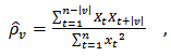 | (7) |
and the lag windows  which are defined in table (1) and spectral density function of autoregressive model, and the consistent estimate of the spectral density function in the formula (2).
 | Table (2). values of the parameter of  |
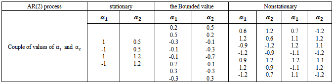 | Table (3). values of the parameters of  |
6) The criterion used to evaluate the kernels performance was the square error (MSE) with the following formula,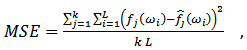 | (8) |
Where  and
and  were defined in (3) and (5) respectively, and
  is the spectrum estimation according to the consistent spectral density function formula in (2).and
  is the spectrum of AR(p), for AR(1) process is,
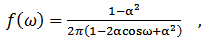 | (9) |
and the spectrum for AR(2) process is,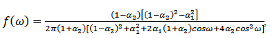 | (10) |
4. The Results Discussion
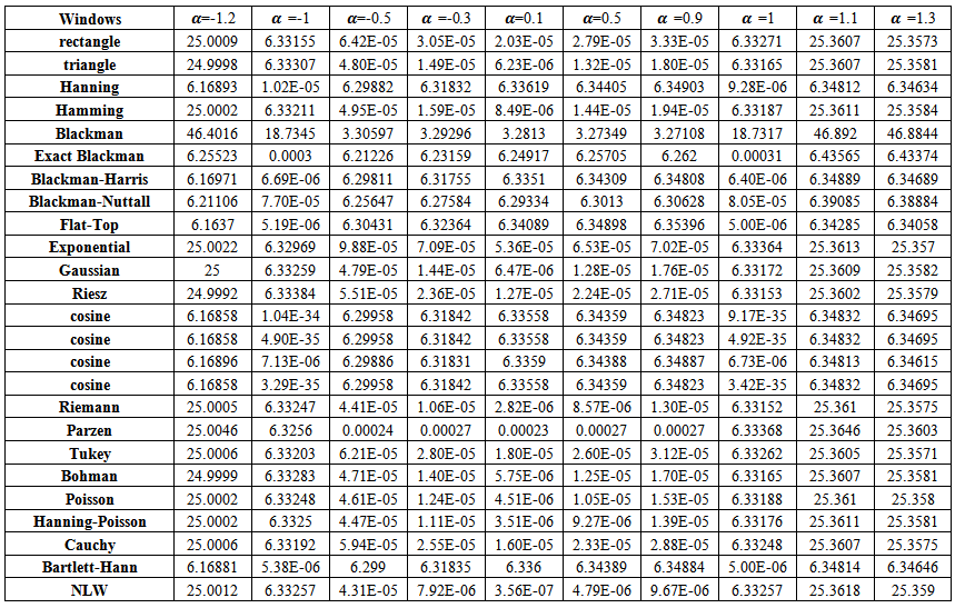
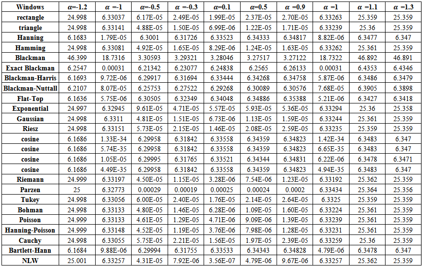
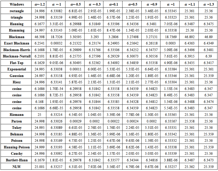
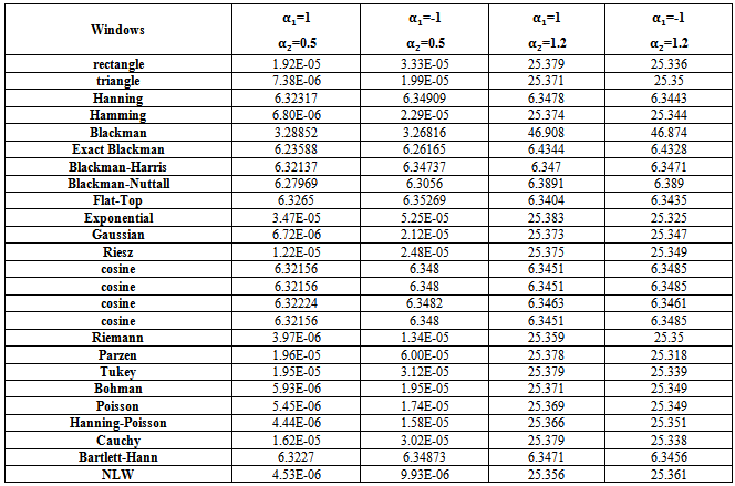
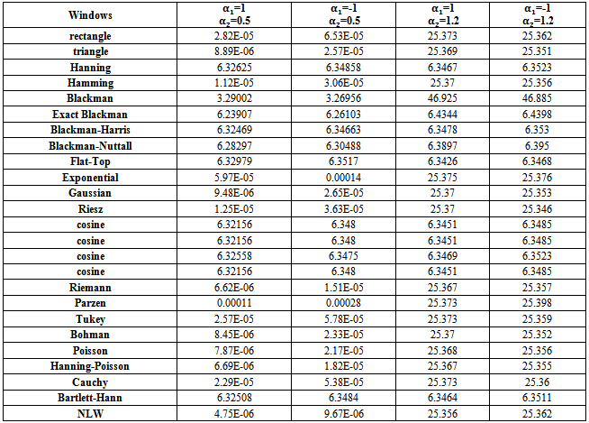
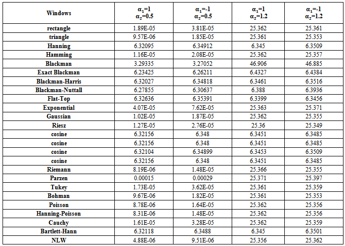
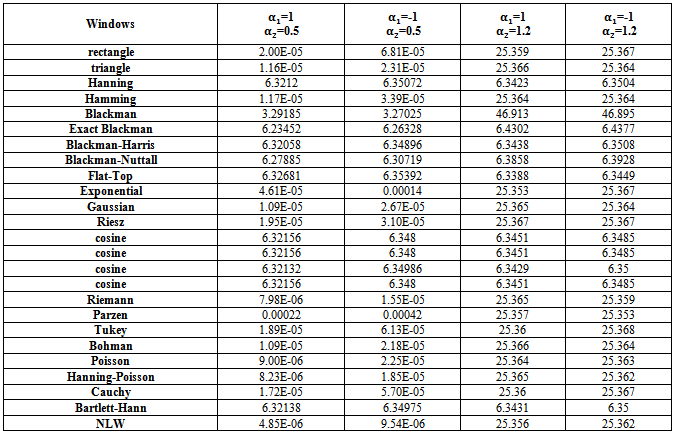
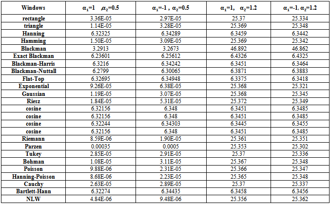
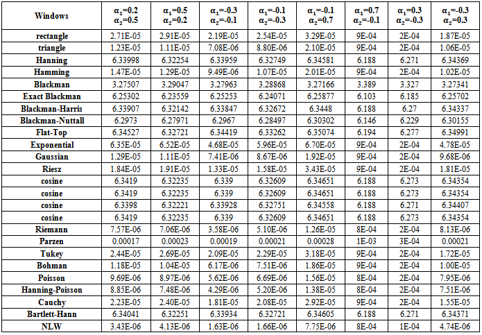
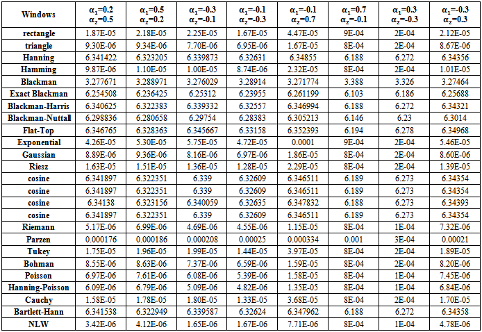
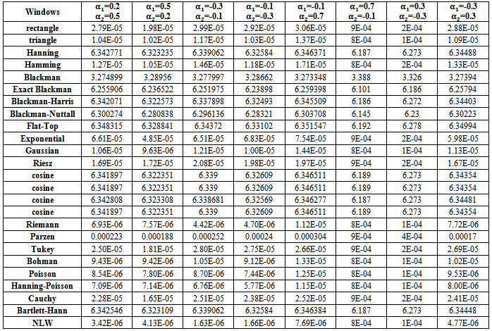
The simulation program was carried out. Tables from (4) to (23) contain the results of MSE Criterion. To discuss the results in efficient way, let us take every process separately,
4.1. The First Order Autoregressive Model AR(1)
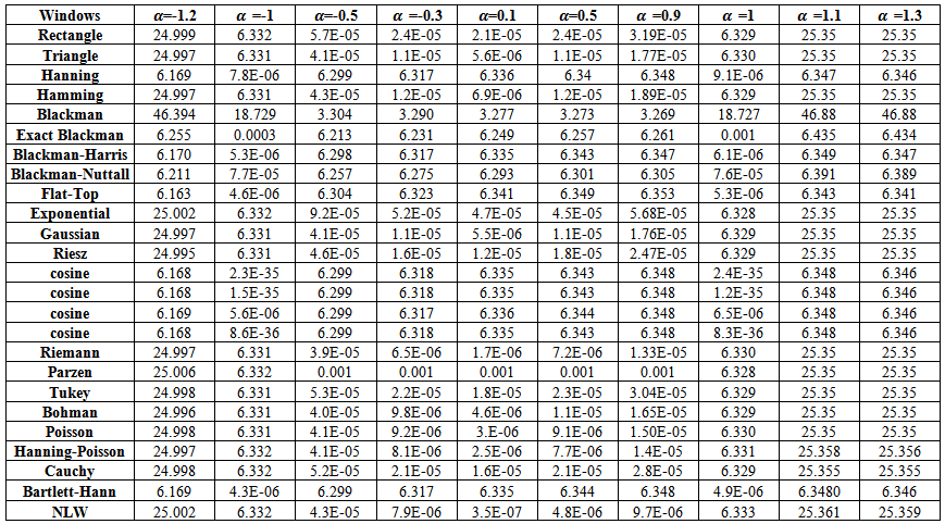
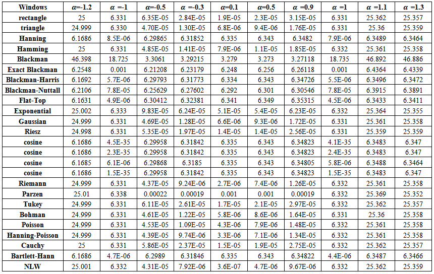
If one noticed carefully, the tables from (4) to (8), resulted from the simulation experiment, he can divide the kernels used according to their behavior to two groups,A - Rectangle, Triangle, Hamming, Exponential, Gaussian, Riesz, Riemann, Tukey, Parzen, Bohman, Poisson, Hann-Poisson, Cauchy, NLW.B - Hanning, Blackman, Exact Blackman, Blackman- Harris, Blackman-Nuttall, Flat-Top, Cosine, Bartlett-Hanning.In the following, some important results, which we reached,1) If one used group (A) kernels, the values of MSE in the nonstationary case 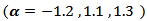 and in the boundary values case
  are clearly, greater than matching values if one used group (B) kernels.2) If one used group (B) kernels, the values of MSE in the nonstationary case
 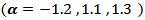 and in the boundary values case
  are very small, and the differences among are very small also.3) If one used group (A) kernels, the values of MSE in the stationary case
  are smaller than matching values if one used group (B) kernels.4) In general, the values of MSE for positive values of
  in the stationary case, are smaller than MSE for negative values except for
  since it is near to the boundary values.5) The Blackman kernel has greatest MSE for all
  and
and  .6) The values of MSE are closed for Triangle and Rectangle kernels for all
  .7) The Flat-Top kernel was the best for the nonstationary cases.8) The cosine5 kernel was the best for the boundary values cases.9) The Riemann kernel was the best only in the case
  and
and  .10) The suggested kernel (NLW) was the best for all other stationary values and all series sizes
  .11) If one used NLW for the stationary cases, There is an extrusive relationship between the values of MSE and
  .
. | Table (4). MSE values of AR(1) spectrum estimation with (n=10) |
 | Table (5). MSE values of AR(1) spectrum estimation with (n=20) |
 | Table (6). MSE values of AR(1) spectrum estimation with (n=50) |
 | Table (7). MSE values of AR(1) spectrum estimation with (n=75) |
 | Table (8). MSE values of AR(1) spectrum estimation with (n=100) |
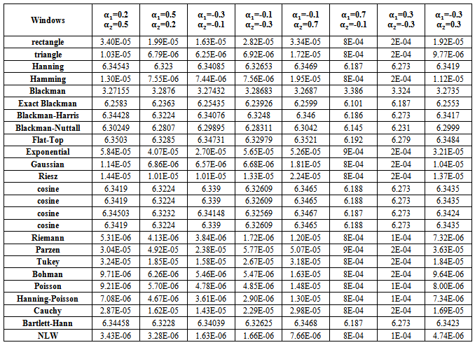
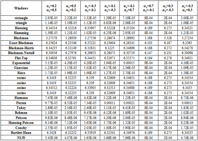
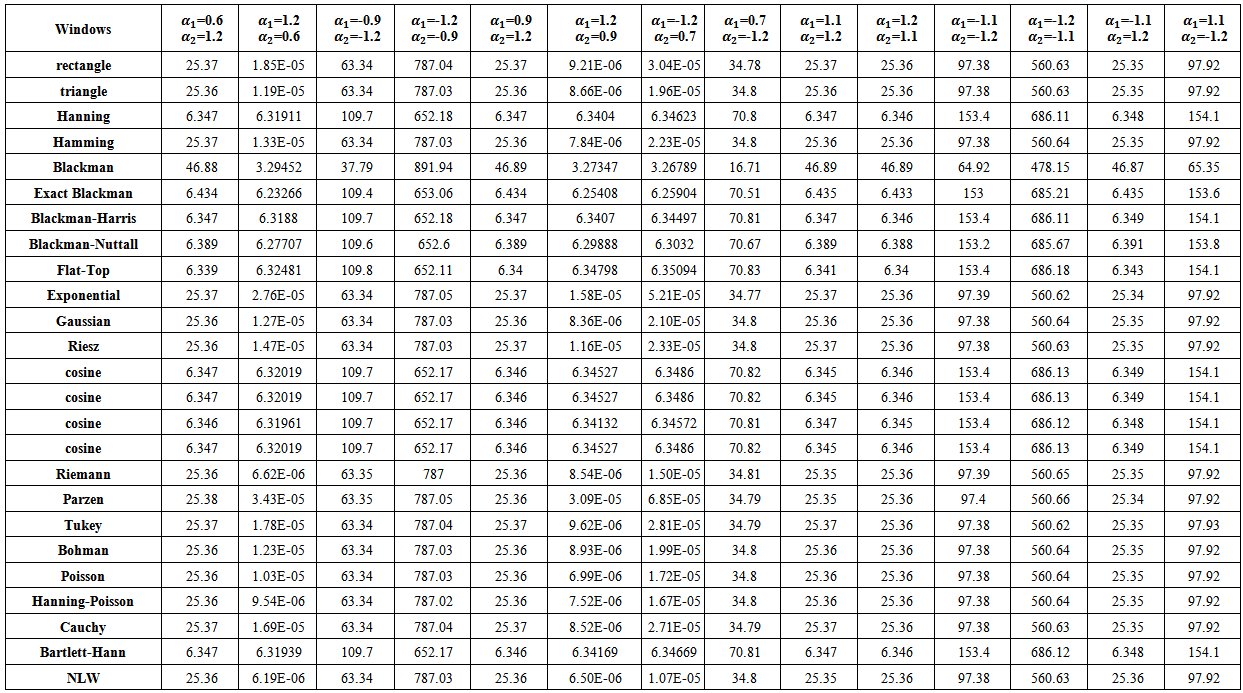
4.2. The Second Order Autoregressive Model AR(2)
If one noticed carefully, the tables from (9) to (23), resulted from the simulation experiment, he can divide the kernels used according to their behavior to three groups,A- Rectangle, Triangle, Hamming, Exponential, Gaussian, Riesz, Riemann, Parzen, Tukey, Bohman, Poisson, Hann-Poisson, Cauchy, NLW.B- Hanning, Exact Blackman, Blackman- Harris, Blackman-Nuttall, Flat-Top, Cosine, Bartlett-HannC- BlackmanIn the following, some important results, which we reached,1 - If AR(2) is Boundary value process (tables from (9) to (13)) , there are different cases,(a) If one used group (A) kernels with the following pairs of parameter values,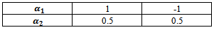 Then(i) The MSE values were very smaller than matching values if one used group (B) or group (C) kernels.(ii) The performance of group (B) kernels was the worst from all kernels according to the MSE criterion.(iii) The performance of the NLW was the best from all other kernels for all series sizes
  .(b) If one used group (B) kernels with the following pairs of parameter values,
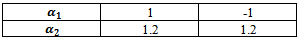 Then(i) The MSE values were very smaller than matching values if one used group (A) or group (C) kernels.(ii) The performance of Blackman kernel was the worst from all kernels according to the MSE criterion.(iii) The performance of The Flat-Top kernel was the best from all other kernels for all series sizes
  .
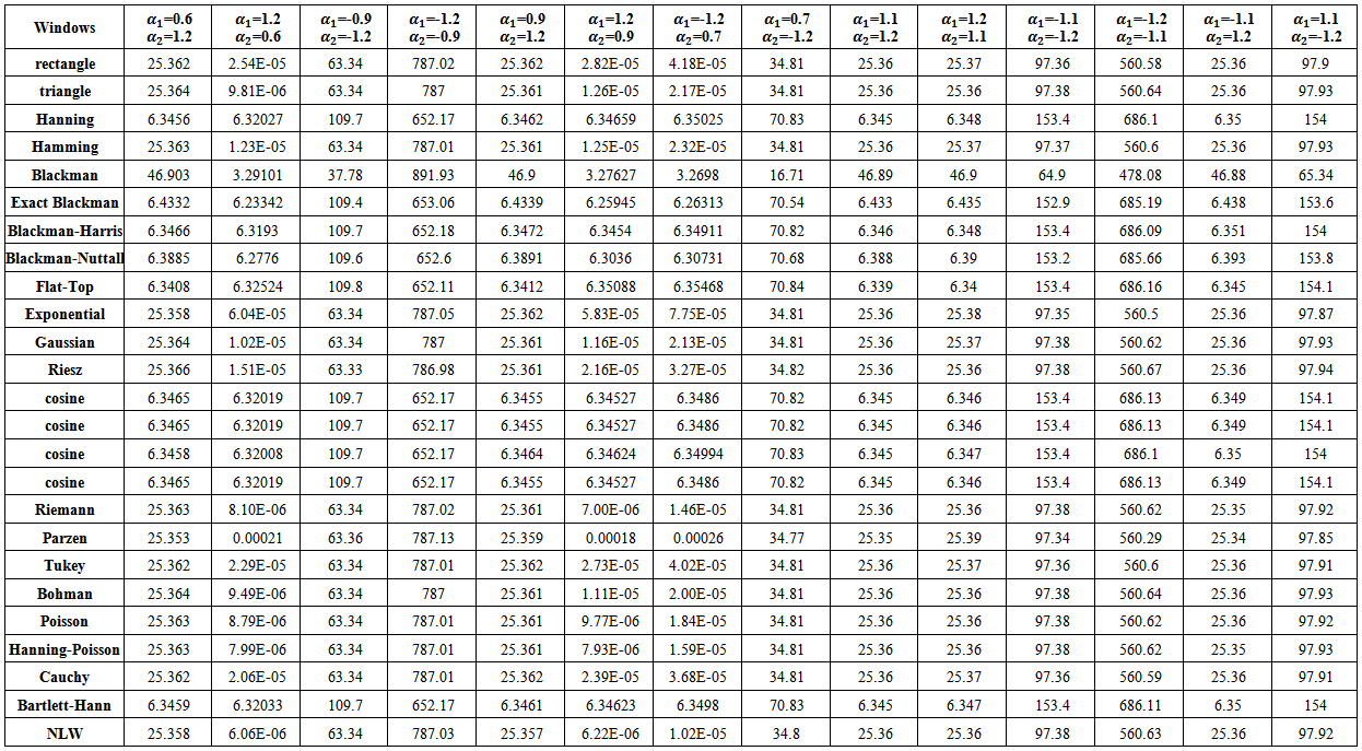
. | Table (9). MSE values of Boundary AR(2) spectrum estimation with (n=10) |
 | Table (10). MSE values of Boundary AR(2) spectrum estimation with (n=20) |
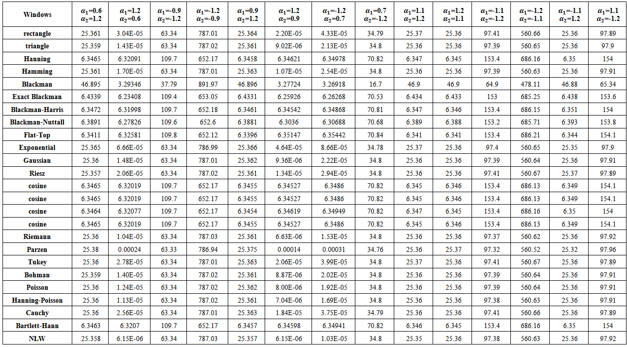
 | Table (11). MSE values of Boundary AR(2) spectrum estimation with (n=50) |
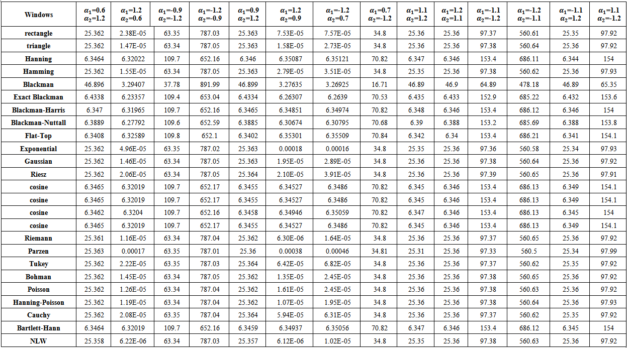
 | Table (12). MSE values of Boundary AR(2) spectrum estimation with (n=75) |
 | Table (13). MSE values of Boundary AR(2) spectrum estimation with (n=100) |
2 - If AR(2) process is stationary (tables from (14) to (18)), there are some important notifications,(a) Generally, the values of MSE are very small, close to zero.(b) The performance of the suggested kernel (NLW) was the best from all other kernels for all series sizes.(c) If one used group (A) kernels, then the MSE values were smaller than matching values if one used group (B) or group (C) kernels.(d) If one used Blackman kernel, then the MSE values were smaller than matching values if one used group (B) kernels.(e) If one used group (B) kernels with  and
and  then the MSE values were bigger than matching values with
  and
and  .(f) If one used group (B) kernels with
  and
and  then the MSE values were bigger than (in simple differences) matching values with
  and
and 
 .(g) If one used group (A) kernels with
  and
and  then the MSE values were smaller than matching values with
  and
and  .(h) If one used group (B) kernels with
  and
and  then the MSE values were bigger than matching values with
  and
and  .(i) If one used group (B) kernels or group (A) kernels with
  and
and  then the MSE values were bigger than matching values with
  and
and  .
. | Table (14). MSE values of Stationary AR(2) spectrum estimation with (n=10) |
 | Table (15). MSE values of Stationary AR(2) spectrum estimation with (n=20) |
 | Table (16). MSE values of Stationary AR(2) spectrum estimation with (n=50) |
 | Table (17). MSE values of Stationary AR(2) spectrum estimation with (n=75) |
 | Table (18). MSE values of Stationary AR(2) spectrum estimation with (n=100) |
3 - If AR(2) process is nonstationary (tables from (19) to (23)), there are different cases,(a) If one used group (B) kernels with the following pairs of parameter values,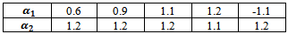 Then(i) The MSE values were smaller than matching values if one used group (A) or group (C) kernels.(ii) The performance of Blackman kernel (group (C)) was the worst from all kernels according to the MSE criterion.(iii) The performance of The Flat-Top kernel was the best from all other kernels for all series sizes
  .(b) If one used group (A) kernels with the following pairs of parameter values,
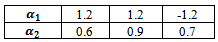 Then,(i) The MSE values were smaller than matching values if one used group (B) or group (C) kernels(ii) The performance of group (B) kernels was the worst from all kernels according to the MSE criterion.(iii) The performance of the suggested kernel (NLW) was the best from all other kernels for all series sizes
  .Generally, the MSE values were very small in all cases.(c) If one used Blackman kernel with the following pairs of parameter values,
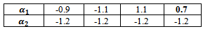 Then,(i) The MSE values were smaller than matching values if one used group (B) or group (A) kernels(ii) The performance of group (B) kernels was the worst from all kernels according to the MSE criterion.(iii) The performance of Blackman kernel was the best from all other kernels for all series sizes
  .Relatively, the MSE values were large in all cases.(d) If one used group (B) kernels with the following pairs of parameter values,
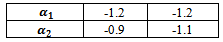 Then,(i) The MSE values were smaller than matching values if one used group (A) or group (C) kernels(ii) The performance of Blackman kernel was the worst from all kernels according to the MSE criterion.Relatively, the MSE values were very large in all cases.
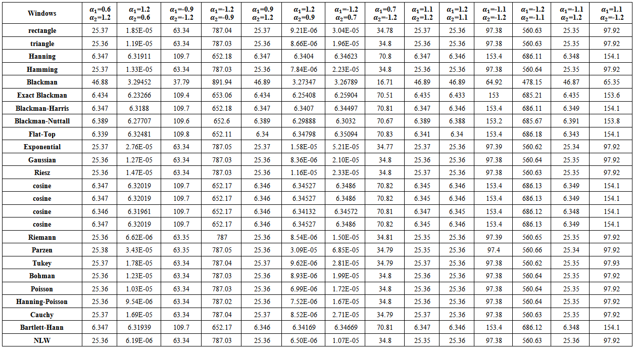 | Table (19). MSE values of nonstationary AR(2) spectrum estimation with (n=10) |
 | Table (20). MSE values of nonstationary AR(2) spectrum estimation with (n=10) |
 | Table (21). MSE values of nonstationary AR(2) spectrum estimation with (n=10) |
 | Table (22). MSE values of nonstationary AR(2) spectrum estimation with (n=10) |
 | Table (23). MSE values of nonstationary AR(2) spectrum estimation with (n=100) |
5. Conclusions and Recommendations
Several important conclusions and recommendations were reached in our thesis.
5.1. Conclusions
The work conclusions can be stated as follows,(a) For the AR(1) process, the Flat-Top kernel was the best for the nonstationary cases, the Cosine kernel was the best for the boundary values cases and the Suggested kernel was the best for all stationary values except in the case  and
and 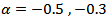 where the Riemann kernel was the best.(b) For the AR(2) process, the kernel vantage were,(i) The suggested kernel was the best for all stationary cases.(ii) For the nonstationary cases, the kernels vantage were as in the following,

 (iii) For the boundary values cases, the kernels vantage were as in the following,
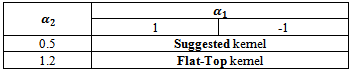 (c) In general, the performance of suggested kernel is very excellent, since it is possible to convert any nonstationary process to stationary process under suitable transformation.
5.2. Recommendations
There are some recommendations can be stated as follows,(a) Use the suitable kernel according to the vantage situations stated in the conclusions section above.(b) Study the performance of the suggested kernel in other cases of ARMA(p,q) process.
References
| [1] | Albrecht, H., 2010, “Tailoring of Minimum Sidelobe Cosine-Sum Windows for High-Resolution Measurements”, The Open Signal Processing Journal, Vol.3, p.20-29. |
| [2] | Box, B. & Jenkins, G. and Reinsel, G., 1994, “Time Series Analysis Forecasting and Control”, Third Addition, Prentice-Hill International Inc, USA. |
| [3] | Abdus Samad, M. , 2012, “A Novel Window Function Yielding Suppressed Mainlobe Width and Minimum Sidelobe Peak”, International Journal of Computer Science Engineering and Information Technology (IJCSEIT), Vol.2, No.2, p.91-103. |
| [4] | Harris, F., 1978, “On the Use of Windows of Harmonic Analysis With the discrete Fourier Transform”, IEEE, vol66, p. 51-83. |
| [5] | Heinzel, G. & Rudiger, A. and Schilling, R., 2012, “Spectrum and spectral density estimation by the Discrete Fourier transform (DFT), including a comprehensive list of window functions and some new Flat-Top windows”, Technical report, Max-Planck-Institut fur Gravitationsphysik, Teilinstitut Hannover. |
| [6] | Hongwei, W., 2009, “Evaluation of Various Window Functions using Multi-Instrument”, VIRTINSTECHNOLOGY.http://www.multi-instrument.com/doc/D1003/D1003.shtml |
| [7] | JOHNSON, M. & TIETJEN, G. and BECKMAN, R., 1980, “A New Family of Probability Distributions with Applications to Monte Carlo Studies”, Journal of the American Statistical Association, Volume 75, NO. 370, p.276-279. |
| [8] | Neave, H. , 1972, “A Comparison of Lag Window Generators”, Journal of the American Statistical Association, Vol. 67, No. 337, pp. 152-158. |
| [9] | Nuttall, A., 1981, “Some Windows with Very Good Sidlobe Behavior”, IEEE Transactions on Acoustics Speech and Signal Processing, vol. 29, NO.1 , p.84-91. |
| [10] | Priestley, M.B., 1981, “Spectral Analysis and Time Series”, ACADEMIC PRESS, USA. |
 Abstract
 Reference
 Full-Text PDF
 Full-text HTML