1. Introduction

The computation complexity of the time-domain adaptive filtering algorithms such as LMS algorithms, gradient adaptive lattice, and Least Square algorithms increases linearly with the filter order[1]-[4], and it is difficult to use such filter in high speed real time applications[5]. The frequency domain LMS algorithms using fast Fourier Transform (FFT) reduces the number of mathematical computations and the orthogonal transform provides more computation counts[6]-[8]. The convergence rate depends on the input autocorrelation matrix and decreases radically with higher input correlation. The transform domain algorithms updated the filter coefficients that can be applied for the case of higher input correlation to obtain higher convergence rate[9][10]. The transform domain adaptive filter achieved rapid convergence of the filter coefficients for non-white input signal with a reasonably lower computational complexity than simpler LMS based system. The gradient based LMS algorithm having convergence rate dependency on the input signal statistics but the LMS-Newton (LMSN) algorithm is another powerful alternatives for larger eigenvalue spread of the input correlation matrix.

The step size (μ) of LMS and the reference signal power play an important role in the stability and convergence of the LMS adaptation process. The fixed value of μ responds to stationary channel, and for the time-varying channel variable step-size LMS algorithm has been proposed to obtain better performance for non-stationary channel[11]-[13]. The Normalized LMS (NLMS) uses variable step-size (μ) algorithm to optimize convergence speed, stability, and performance. The time-variable step-size (μ) is implemented based on the power estimation of the input signals[14]. The larger μ is used for non-stationary and smaller μ is used for stationary without considering the convergence rate[15][16]. Further, modification on NLMS is proposed named as VS-NLMS in which μ is decided by the estimation of input signals, and it achieves a faster convergence rate with maintaining the stability of the NLMS[17]. The proposed VS-LMS with time-varying step-size (μ) improves the output signal to noise ratio (SNR) and the convergence speed. A new type of criteria is proposed using output error with step-size value (μ) from a big value α₂ and smaller one α₁ to provide faster tracing speed and smallermisadjustment[18]-[20]. The stability and convergence properties of transform - domain LMS algorithm has been investigated in[21], the authors also analyzed the effects of the transforms and power normalization in various adaptive filters for both first order and second order AR process. In the same work they stated that the power normalization increases the difficulty for analyzing the stability and convergence performance. The LMS-Newton algorithm avoids the slow convergence of the LMS algorithm for highly correlated input signal[15], this property should be very useful in DWT-LMS algorithm and is used in this work.

In[21]-[23], the authors analyze the transform-domain adaptive filters with discrete Fourier transform (DFT), discrete Cosine transform (DCT), discrete Hartely transform (DHT), and discrete Sine transform (DST) for first-order and second-order AR input process with their stabilities and convergence performance for input power normalization. The result of the work[24] shows that the DCT-LMS and DST-LMS provides the better convergence performance for both first and second order AR process than the DFT-LMS and DHT-LMS. In this paper, we analyze the Discrete Wavelet Transform (DWT) in adaptive filtering algorithm in form as DWT-LMS Newton adaptive filters for both first order and second order AR process to enhance Misadjustment to measure the steady-state convergence, and MSE performance. This paper also discuss the design of the DWT-LMS for the time-varying AR process, the time-varying block by block basis data is processed by using ε-decimated DWT algorithm. The simulation study in our work shows that SWT-LMS Newton adaptive filter provides better stability, misadjustment, and convergence performances than that of DFT-LMS and DCT-LMS for both first order and second order AR process[23].

2. Analytical Form of Transform-Domain LMS-Newton Algorithm

The LMS-Newton algorithm estimates the second order statistics of the wide-sense stationary signal. The algorithm avoids the slow convergence of the LMS algorithm for highly correlated input signal. The LMS-Newton algorithm minimized the MSE at instant (n+1) if[15]

(1)

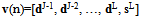
where μ is a convergence factor that is used to protect the algorithm form divergence due to noisy estimate of input auto-correlation matrix R and the gradient vector g_w (R). is the estimation of the auto-correlation matrix, namely, R≈E[u(n)u^H(n)], u(n) is the input signal vector. The unbiased estimate of R for stationary input signal is as:

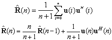(2)

Here, the Hermitian transpose (H) is used for input complex vector. Again, the estimation on both sides of (2) gives,

(3)

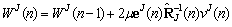
The estimation for R requires infinite memory location for large n. Another form of estimation of the autocorrelation matrix by introducing a small factor α, in the range 0<α<0.1 to provide the good balance of input signal information. The resulting equation to calculate the inverse matrix that is required for LMS-Newton algorithm can be given using the Matrix inverse Lemma as[21]:

(4)

with α(n)= α. The coefficient updating formula (1) can be written using the estimate of gradient vector as[22]:

(5)

where,

(6)

d(n)=desired signal, w(n-1)=weighting vector at iteration n-1; =δI (δ is positive constant less than 0, and I is unity matrix); w (0) =[0 0 0 . . . . . . .]^T

The transform domain LMS transformed the input signal vector u(n) in a more convenient vector s(n), s(n)=Tu(n), where TT^H=I, the transform matrix of following form as:

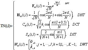(7)

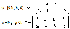
where, i, l=0, 1,……, N-1; k_i=1/√2 for i=0 and 1 for otherwise, and are wavelet function and scaling function respectively. The autocorrelation matrix for the transform-domain input signal vector s(n) is given by:

(8)

The misadjustment of the adaptive filter is the ratio of the excess mean square error (MSE) and minimum MSE in the steady-state which is a measure of the noise in the filter output due to fluctuations in the filter coefficients. The formula for misadjustment based on the expression for weight noise covariance is given as[24][25]:

(9)

The result can be used for the transform-domain LMS adaptive filters and is given by:

(10)

Stability can be determined by the condition of M of finite value and we must choose μ within the range 0<μ<1/tr (R) ; for the case of (9), and 0<μ<1/tr R_s; for the case of (10).

3. Wavelet Packet Transform Based LMS Algorithm

The wavelet packet transform of the signal x(n) can denoted as[25][26]:

(11)

y(n) is the M1 wavelet packet transform signal vector, V_p the 2^J2^J wavelet packet decomposition for the J series as follows[27]-[29]:

(12)

The LMS algorithm is used as: r(n)=W^T(n)y(n)

where W is the weighted vector of LMS algorithm, r(n) is the output signal of LMS. The error of the filter is as:

(13)

where d(n) is the desired signal, and we have:

(14)

where μ is the step-size parameter.

3.1. Algorithm Performance Analysis

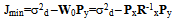
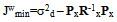
The cross-correlation vector P_y between the desired signal d(n) and the wavelet packet transform signal y(n) is as:

(15)

Where, P_x is the cross-correlation between the input signal x(n) and the desired signal d(n). The auto-correlation matrix R_y of the wavelet packet transform signal is as:

(16)

where R_x is the autocorrelation matrix of the signal x(n). The wiener optimal solution of wavelet packet domain is as:

(17)

Here, W₀=R^-1_xP_x; the time domain wiener solution. The MSE of wavelet packet domain is derived in appendix A and is given as:

(18)

The minimum error in the mean square error is as:

(19)

The minimum MSE in wavelet domain is equal to that of time domain and can be written after further solving (19) and can be given as[30][31]:

(20)

3.2. Convergence Analysis of Wavelet Transform Domain LMS Adaptive Filter with AR Process

AR(P) model for univariate time series are Markov process, and P^th order AR process to generate the data y_t is as:

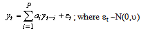(21)

where a_k; k=1, 2, 3, , P are AR coefficients and ε_t a white sequence with ε_t ⊥ε_s for t≠s. The M order N×N autocorrelation matrix R_N can be given according to[23] as:

(22)

Here,

(23)

where, c₁, c₂, , c_M are constant and ρ_k for all k are the M poles of low pass filter with ρ_k∈[0, 1] for all k.

3.2.1. Eigenvalue Spread for First Order AR Process

The first order Markov signals can be obtained by passing a white noise through a one-pole low-pass filter. The N by N autocorrelation matrix of AR (1) or Markov-1 process is obtained from (23) as:

(24)

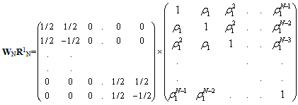
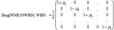
The autocorrelation matrix in the wavelet domain for AR (1) process is the autocorrelation matrix of the Markov-1 process of the wavelet transform domain input signal of the same parameter ρ that is: ; where W is the N×N order wavelet transform matrix. Now, putting the value of the wavelet transform matrix from (B. 10) of appendix-B, we have the following form as:

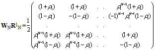
(25)

The Toeplitz matrix defined by the first row of (25) as:

(26)

Now, substituting the corresponding elements from (25) into (26) we have:

(27)

for odd value of l

(28)

for even value of l

The power spectrum of the wavelet domain input AR(1) process can be written as[26]:

(29)

where, . Now, from (29) we have the power spectrum of the form as:

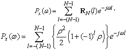(30)

Now, considering a=0.5{1+(-1)²ρ}, we have (30) in the form as:

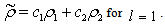
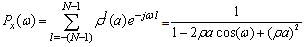Again considering ρ₁=ρa, we have above equation in the following form as:

(31)

Maximum value of the eigenvalue when cos(w)=1, we have

(32)

The minimum value when cos(w)= −1, and we have

(33)

The Eigenvalue spread of the following form

(34)

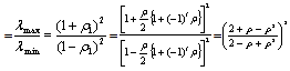
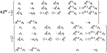
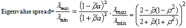
3.2.2. Eigenvalue Spread for Second Order AR Process

The characteristic equation for second order AR (2) process is given as[32]:

(35)

The pole of the filters ρ₁, and ρ₂ is defined by the characteristics equation with the following form of transfer function as:

(36)

The N×N correlation matrix of the AR(2) process can be defined as:

(37)

Where,

(38)

(39)

The following matrix is defined as[25]:

(40)

Where,

(41)

and W_N is the N^th wavelet transform matrix defined in (B. 10) of appendix-B. The numerical value of the matrix D_N of (40) has been calculated in appendix-C and is given as:

(42)

if c=c₁+c₂, and s=c₁ρ₁+c₂ρ₂ then (44) can be written as:

(43)

Now, we compute the simple matrix;

(44)

The wavelet transform-domain autocorrelation matrix R^DWT_N for AR(2) process can be written in the following form as:

(45)

(46)

where, ρ_a=1+ρ₁, ρ_b=1-ρ₂, and ρ_x=1+ρ₂, ρ_y=1-ρ₂. The power spectrum of the input with AR(2) process can be written as:

(47)

Now, we can find R^DWT_N(l,l) from (44) and is given as:

(48)

If ; l=0, 1, , N-1, the (50) can be written as:

(49)

where, . Now, (50) can be written as:

(50)

Eigen value maximum when cos(ω)= −1 and minimum when cos(ω)=1. The Eigenvalue spread is given as:

(51)

where,

4. Structure of Wavelet Transform LMS Algorithm

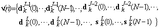
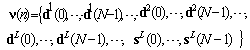
Signal in most of engineering applications are non-stationary, and Fourier transform encountered difficulty to analyze the time-frequency property[33][34]. The wiener filter is assumed to be stationary but the stationary assumption of the noisy signal cannot completely satisfied in many applications[35]. The SWT domain signal vector v(k) in the matrix form can be expressed as:

(52)

where, x(k)=[, x(k+1), x(k), x(k-1), ]^T , ψ is the wavelet transform matrix whose row vector is ψ_mn as:

(53)

The SWT-transformed signal vector v(k) can be expressed in the following form as:

(54)

The smooth and details components at level j can be expressed as:

(55)

The low pas filter H and high pass filter G denoted by the sequence {h_n}_n∈_z and {g_n}_n∈_z with g_n=(-1)ⁿh_1-n; where h_n’s satisfy the orthogonaligy condition h_nh_n+2j=0; j=0, 1, 2, ., SWT on N samples of signal x(n) yields[35]:

(56)

where, x(n)={x₀[0], , x₀[N-1], , x_k[0], , x_k[N-1], , x_k-1[0], , x_k-1[N-1]}. The SWT provides the same length of both smooth and details components and this property is very useful in time-varying application of wiener filter in block by block basis. The SWT-domain based LMS algorithm provides the system output signal y(k) that can be represented in the following form:

(57)

where, J=1, 2, , L; L is the level of decomposition. The weighting vector for each level can be denoted as:

(58)

The SWT domain (v(n) ) of the input signal x(n) as in (57) having the following form as:

(59)

The SWT based LMS algorithm according to (5) can be represented as:

(60)

where, e^L(n)=v^L_d(n)-W^L(n-1)v^L(n)

v^L_d(n)=L level SWT domain signal of the desired signal d(n), in vector form v^L_d(n )=[ v^L_d(0), v^L_d(1), , v^L_d(N-1)].

The convergence factor and misadjustment for each level of the SWT domain signal is governed according to the algorithm as discussed in section 2 of this paper. The MSE cost function of each level can be written in the following form as:

(61)

5. Result

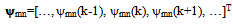
The misadjustment of the adaptive filter measures the amount of noise in the filter output and increases with the step-size parameter. Lower amount of misadjustment indicates the better denoising performance of the filtering algorithm. Let us consider a multi-tone signal of the following form as:

(62)

The toeplitz matrix R_y of the autocorrelation matrix of the multi-tone signal y(n) in (62) before any transformation is shown in Fig. 1(a). The toeplitz matrix after application of DCT and DWT in the multi-tone signal y(n) is shown in Fig. 1(b) and Fig. 1(c) respectively. The misadjustment curve in Fig. 1(d) shows that the misadjustment increases of the three cases as input toeplitz matrix, DCT based input toeplitz matrix, and DWT based input autocorrelation matrix. The DWT-based curve shows the better performance because it provides less misadjustment value for all values of μ than other two.

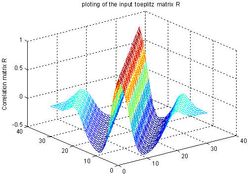Figure 1(a). Autcorrelation matrix of the input multi-tone signal without any tranformation

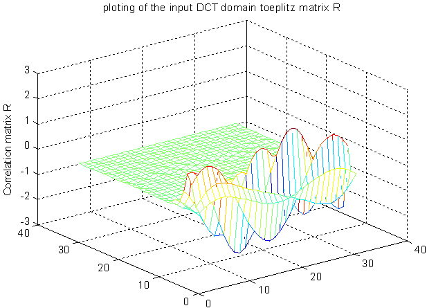Figure 1(b). Autocorrelation matrix of the DCT transformed based multi-tone signal

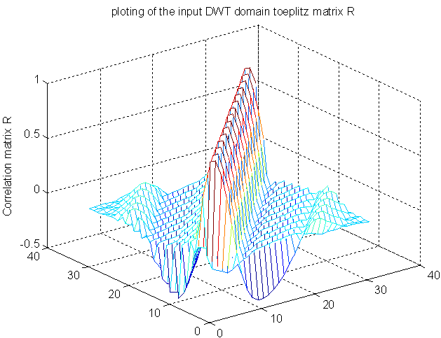Figure 1(c). DWT based autocorrelation matrix of the input multi-tone signal

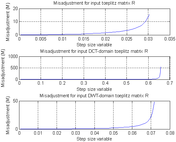Figure 1(d). Misadjustment result of input autocorrelation matrix, DCT and DWT based input autocorrelation matrix

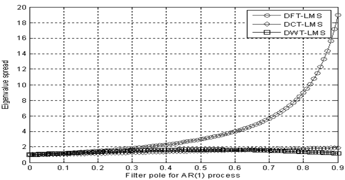Figure 2. Eigenvalue spread of DFT-LMS, DCT-LMS, and DWT-LMS for AR (1) input process

The eigenvalue spread of DFT-LMS and DCT-LMS for AR(1) process is shown in Fig. 2, details of the work has been discussed in the work[23][36]. The eigenvalue spread of DWT-LMS analyzed in this paper with the same procedure is also shown in Fig. 2, the result shows that DWT-LMS achieves the smaller eignenvalue spread than DFT-LMS and DCT-LMS at some upper region of the area of (ρ). Hence, DWT-LMS gives the best convergence performance for the AR(1) input process. The eigenvalue spread for DFT-LMS and DCT-LMS for AR(2) input process has been analyzed in the work[25] and the result is also shown in Fig. 3(a) and Fig. 3(b). In the work[25], DCT-LMS achieves the smaller eigenvalue spread than other and provides the best convergence performance for the AR(2) process.

The autocorrelation matrix R_N for LMS with AR(2) process without any transformation is calculated in (37), and the same calculation for the multi-tone siganl is calculated in this paper with ρ₁ and ρ₂, and the 3D-plot of the matrix is shown in Fig. 4(a).

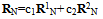
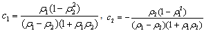
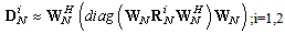
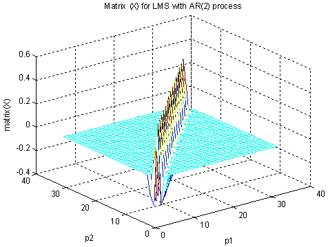
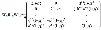
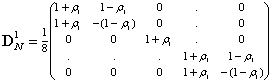
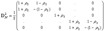
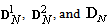The matrix in (41) and (40) after applying DWT in the input AR(2) process is shown in Fig. 4(b), Fig. 4(c), and Fig. 4(d) respectively. Now, we compute the matrix 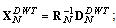where R_N is given in (37) and is given in (43) and plotted in Fig. 4(d). The distribution of is shown in Fig. 5(a) for the sample value of N=30, the result shows that most elements of is very close to zero and the only the diagonal elements having values close to 0.6. The distribution of is very important factor to compute the eigenvalue spread of the autocorrelation matrix V_N; that obtained after DWT.

Figure 3(a). Eigenvalue spread of DFT-LMS for second-order lowpass AR process

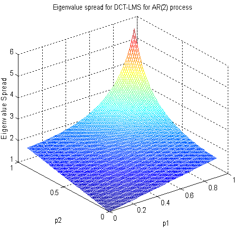Figure 3(b). Eigenvalue spread of DCT-LMS for second-order lowpass AR process

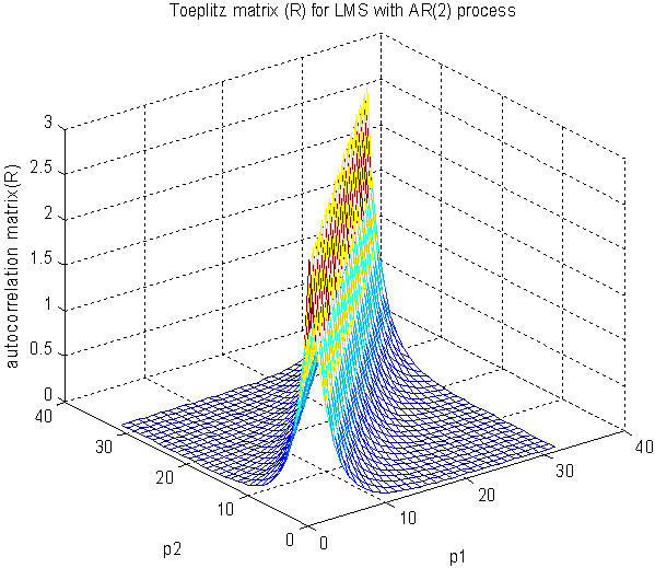Figure 4(a). Autocorrelation matrix RN before any transform for AR(2) input process

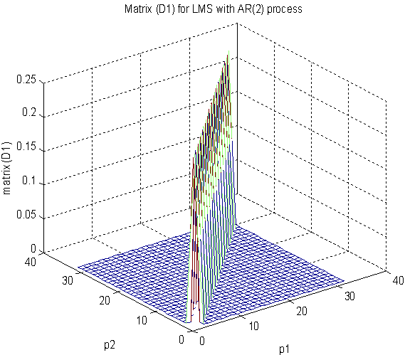Figure 4(b). Matrix after DWT in the AR(2) process

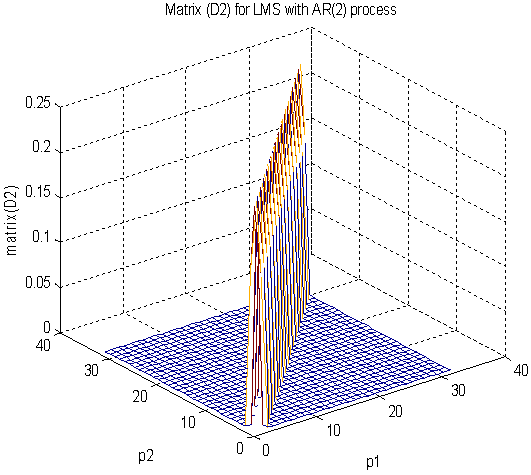Figure 4(c). Matrix after DWT in the AR (2) process

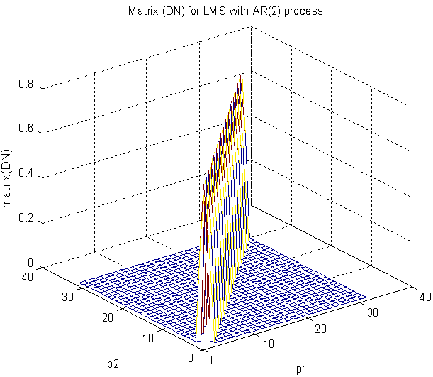Figure 4(d). Matrixn DN after DWT in the AR(2) process

Figure 5(a). 3D plot of the matrix involved in DWT-LMS eigenvalue spread calculation

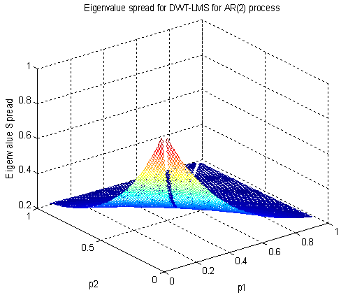Figure 5(b). Eigenvalue spread of DWT-LMS for second-order lowpass AR process

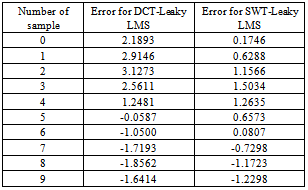
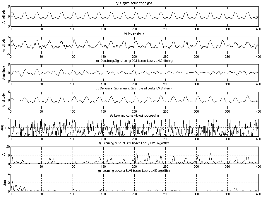Figure 6. Denoising performance of DCT-Leaky LMS and SWT-Leaky LMS for AR(2) process

The convergence relation for DWT-LMS can be obtained from (51) for real roots of ρ₁, ρ₂<1 with second-order input case. The eigenvalue spread can be plot for DWT-LMS with given real or complex values of ρ₁, and ρ₂. The 3D plot of the eigenvalue spread of DWT-LMS is in Fig. 5(b), the result shows that the value converges to zero when both roots deviate from the origin. The eigenvalue spred of DFT-LMS, DCT-LMS, and DWT-LMS for second-order AR process as in Fig. 3(a), 3(b), and 5(b), and the result shows that DWT-LMS provides the best convergence performance among them. Hence, the lower value of the eigenvalue spread of DWT-LMS provides the lowest noise term in the output of the denoise signal. To support the above analytical result, the signal in (62) is passed through a 2^nd order AR filter as given below:

(63)

where, v(n) is white gaussian noise with mean zero and variance σ₂; a=[1 0.5 0.33] is the AR coefficients. The original multi-tone and output of the AR filter as noisy signal is shown in Fig. 6(a) and Fig. 6(b). The DCT algorithm as in[40] is used in Leaky LMS-Newton adaptive filter[36] which is known as DCT-Leaky LMS-Newton algorithm which is actually same as LMS with better denoising performances. In this paper. the AR(2) output signal is passed through DCT-Leaky LMS and SWT-Leaky LMS with considering μ=0.01 and γ=0.1, the value of µ is considered depending on the stability condition, details of the mathematical analysis is discussed in sectin II. The denoising signal of DCT-Leaky LMS and SWT-Leaky LMS is shown in Fig. 6(c) and Fig. 6(d), the result shows that SWT-Leaky LMS provides better denoising performance than DCT-Leaky LMS. The error of the denoised signal from the actual is given in the below Table-1. From the table it can be concluded that SWT-Leaky LMS provides more denoising than DCT-Leaky LMS for each sample value.

Table 1. Denoising Error of DCT-Leaky LMS and SWT-Leaky LMS

The learnign curve J(n) or MSE of both DCT-Leaky LMS and SWT-Leaky LMS with the same parameter through the same noisy channel is shown in Fig. 6(f) and Fig. (g). From the result it is shown that the maximum value of the learning curve of SWT-Leaky LMS is close to 2 at initial sampling point an it converge to zero after 10 sample points, in the other hand DCT-Leaky LMS provides high value of J(n) as upto 10 and it repeated to the maximum after 30 sample points. So, SWT-Leaky LMS provides better convergence performance than DCT-Leaky LMS algorithm.

6. Conclusions

The stability and convergence performance of DFT-LMS, DCT-LMS, DHT-LMS, and DST-LMS has been analyzed in details in work[25], and the result shows that DCT-LMS and DHT provides better convergence performance than other. In this work, we have designed DWT-LMS Newton adaptive or SWT-LMS Newton adaptive, or in simply DWT-LMS or SWT-LMS adaptive filtering algorithm and the performances is compared with the DCT-LMS adaptive filtering algorithm for first-order and second-order AR process as developed in the early work[25]. From the comparison result it is shown that DWT-LMS provides better misadjustment, convergence,and denoisingperformance than that of DCT-LMS adaptive filtering algorithm for both AR(1) and AR(2) process. For example, if ρ=0.8 then eigenvalue spread of DCT-LMS is 1.8 and for DWT-LMS is 1.37 for AR(1) process. The eigenvalue spread of DCT-LMS is 2.63 and for DWT-LMS is 0.25 for ρ₁=0.59 and ρ₂= 0.79 respectively with AR(2) process. From talble-1, it is also concluded that SWT-LMS provides less denoising error in each sample value than DCT-LMS adaptive algorithm. Hence, the DWT-LMS provides better misadjustment, convergence or eigenvalue spread, and denoising performance than others as presented in work[25]. In future the SWT-LMS algorithm can be applied for higher order AR process and other type of input process like MA and ARMA process.

APPENDIX A: MSE of Wavelet Packet Domain Signal

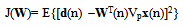
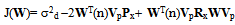
J(W)=E{e²(n)}=E{[d(n) −r(n)]²}=E{[d(n)-W^T(n)y(n)]²}

The error function in wavelet domain can be written by replacing the input signal in wavelet transform domain as:

(A.1)

J(W)= E{[d(n) −W^T(n)V_px(n)]×[d(n)-W^T(n)V_px(n)]}

J(W)=E{d²(n)}−2W^T(n)V_pP_x+W^T(n)V_pE{d(n)x(n)}+W^T(n)V_pE{x(n)x^T(n)}W(n)V_p

Now, E{d²(n)}=σ²_d is the variance of the desired signal d(n).

P_x=E{d(n)x(n)}; the cross-correlation between d(n) and x(n)

P_y=V_pP_x; Cross-correlation vector in wavelet domain

R_x=E{x(n)x^T(n)}; autocorrelation matrix of x(n)

R_y=V_pR_xV_p; autocorrelation matrix in wavelet domain

W(n)=R^-1_yP_y; filtering weighting vector in wavelet domain

Substituting those parameters we have the solution as:

(A.2)

APPENDIX B: Algorithm in Generating a Wavelet Matrix

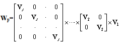
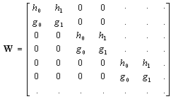
Let us assume W be an N by N matrix of the following form:

(B.1)

Where I is also N by N unity matrix, the alternative form of (B.1) can be written as:

(B.2)

Where δ_i for i=1, 2, , N is the i^th column of I. Equation (B.2) implies that the wavelet transform on δ_i; i=1, 2, , N provides N column vectors and the vectors form a wavelet matrix. The 1 scale wavelet transform of a column vector x of length N can be expressed as[31][38]:

(B.3)

The two scale wavelet coefficients can be represented as:

(B.4)

where W’₂^(N) can represented of the following form as:

(B.5)

where W₁^(N) and W₁^(N/2) corresponds to 1 scale wavelet transform matrix of length N and N/2. Now, the 2 scale wavelet transform matrix for the input vector x can be represented by integrating (B.4) and (B.5) as:

(B.6)

A k scale wavelet transform matrix can be generated by the procedure in (B.6) and can be represented in the following form as:

(B.7)

Now, assume the high pass and low pass filter response of the form, h=[h₀, h₁, , h_m-1], and g=[g₀, g₁, , g_m-1], then we have the wavelet two functions of the form as:

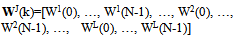
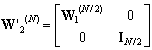
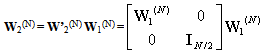
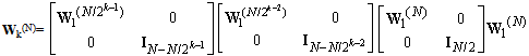
The first scale matrix W₁^(N) can be written in the form as:

(B.8)

The transform matrix for the Haar wavelet can be written of the form as[39][40]:

(B.9)

In the case of Haar transform the scaling and wavelet values have been given in[41] with[h₀, h₁]=[1/2, 1/2] and[g₀, g₁]=[1/2, -1/2]. The wavelet transform matrix can be written as:

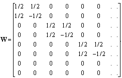(B.10)

APPENDIX C: Determination of Wavelet Domain Auto Correlation Matrix with AR(2) Process

Using (B.10) and (39), we have

(C.1)

(C.2)

(C.3)

(C.4)

Again, D¹_N= W^H_N{ Diag(W_NR¹_NW^H_N) W^H_N }, and we have the numerical value as:

(C.5)

Similarly, D²_N= W^H_N{ Diag(W_NR²_NW^H_N) W^H_N }, and we have the numerical value as:

(C.6)