1. Introduction

High frequency oscillation (HFO) is a short rhythmic brain wave consisting of at least three oscillations in the frequency range 80-500Hz[1], and can be clearly distinguished from background activities[2]. HFOs are divided into Ripples 80-250Hz and Fast Ripples (FRs) 250-500Hz[1,2,3,4,5,6]. HFOs can be recorded with invasive EEG procedure using commercial subdural grid/strip and depth electrodes. Invasive EEG can give an accurate reading of neural activities recorded at the brain surface level and within the brain volume[7] for patients with intractable epilepsy. Recent studies reported that HFOs bursts in the band of 40-200Hz[8] and 80-150Hz[9] can also be recorded on the scalp EEG.

HFOs are more specific and accurate than spikes/sharp waves to delineate the seizure onset zone (SOZ)[6,10]. HFOs were discovered in epileptic rats and patients with epilepsy[1,3,4] and may be encountered under physiological [11] or under pathological conditions[6,11]. It has been reported that a large proportion of HFOs co-occur with spikes[5], and can also occur independently in non spiking channels[6,12]. Postsurgical study[13] showed a good correlation between surgical outcome and removal of channels with high HFO rates. Rates[5,6,12], powers[5], and durations[6,12] of HFOs were higher within than outside the SOZ. Moreover, HFOs bursts mark epileptogenicity rather than lesion type[14]. In summary, HFOs bursts seem to be a reliable biomarker of epileptogenic tissue capable of producing seizures and can provide some useful information for understanding of the fundamental neural mechanisms underlying epileptic phenomena.

Visual analysis of HFOs was previously provided a good and adequate understanding[5,6] of the relation of HFOs with epilepsy. However, this manual procedure is tedious especially for analyzing long and multi channels EEG recordings, time-consuming (it takes about 10 hour to visually mark HFOs in a 10- channel/10-min recording[15]), inevitably subjective. It is also possible that some actual small HFOs oscillations escape visual inspection[16]. Visual processing of HFOs may also be subject to error prone and requires a great deal of mental concentration and qualified/experienced reviewers. Thus, automated and reliable detection of HFOs may be more useful, fast, consistent, and objective than the visual identification. Moreover, automated software is crucial and necessary for the systematic study and investigation of HFOs in large scale research. A comparison of existing detectors on the same database is important to analyze their performance in terms of correct/false detection rate, and for comparing their robustness of detection.

In the present framework, we firstly improved three existing HFOs detectors, which are based on time frequency techniques. We then compared their performance to that of a human reviewer using two commonly metrics: Sensitivity and False Discovery Rate (FDR). The first method is based on Complex MORLET Wavelet (CMV). The second is derived from Matching Pursuit (MP), and the third uses Bumps Modeling Technique (BMT).

The structure of the paper parts is ordered as follows: Section.1 presents Introduction. Section.2 describes the clinical database. In section.3, the various details of the mentioned methods are provided. Section.4 describes visual marking of HFOs and section.5 presents performance metrics. Section.6 presents the discussion and the comparison of different methods. Last section presents conclusion and our outlines future work.

2. Clinical Database

The clinical database used in the present study was recorded using the Harmonic system (Stellate) at the Montreal Neurological Institute and Hospital (MNI), Canada. The data was low-pass filtered at 500 Hz and subsequently sampled at 2000 Hz. Then, sampled data was quantized using a 16 bit analog-to-digital converter. In order to avoid the risk of focusing our study on a particular data, the used channels were chosen based on the following criteria: clear presence of interictal HFOs upon initial review is firstly controlled. Second, both channels with active and rare HFO events were considered. Third, a group of three consecutive patients with intractable epilepsy was considered for the current study. In the last, channels contain different background level were selected. All patients gave informed consent in agreement with the research ethics board of MNI.

3. Methods

Time-frequency (TF) based methods are a combination of both theory and information. TF methods have been used extensively in the processing and analysis of non stationary signals, as found in a wide range of application including biomedical engineering. Their advantage can be resumed as follows: localization of information about both time and frequency together, automated classification of specific patterns based on their frequency components. They allow determining of coupling relationships among frequencies, amplitudes and phases of signals, which can provide insights about some underlying physiologic, pathologic process of many neurological diseases like Epilepsy, Parkinson and Alzheimer. TF based methods also allow measuring the reproducibility in signals and interpretation of models that may reflect pathological and physiological behavior in neuroscience.

Details for HFOs detection using the mentioned methods are provided below:

3.1. Detection of HFOs based on Complex MORLET Wavelet (CMW Method)

For HFOs detection based on CMW, power coefficients is firstly computed using the complex MORLET wavelet [2,17].

is defined as follows:

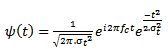(1)

Where represents the central frequency of the mother wavelet . The standard deviation of the gaussian window used here is set to 1. The wavelet family is chosen so that the ratio of its center frequency to bandwidth is equal to 7, which corresponds to a good HFOs legibility and lead to the highest correlation coefficients with HFOs events. This choice according to the following equation:

(2)

Where, the Fourier spectrum of the complex MORLET wavelet is a Gaussian with standard deviation . The relationship between and is defined as follows:

(3)

The mother wavelet defined above in equation.1, can be scaled by a factor and translated by an amount b in time as follows:

(4)

is known as a daughter wavelet. Scale is related to a pseudo-frequency , according to the following relationship:

(5)

Where is the sampling period and is equal to (7/2π) in our case. The wavelet power is then computed as follows:

(6)

is computed from wavelet power by transforming scale a into integer pseudo-frequency f using equation.5 and replacing b by the sample Pseudo frequency values ranging from 80Hz up to 500Hz with a step of 5Hz were used. represents a three-dimensional map described in time (x-axis), pseudo-frequency (y-axis), and coefficient values (z-axis) in dB. Afterwards, to improve the localization of HFO events and to reduce noise impacts, time frequency map is subsequently smoothed using a robust smoothn function described in[18]. More details about this function are available at:

http://www.biomecardio.com/matlab/smoothn.html.

If an HFO is present, then it will create a local maximum (also called burst) in the power coefficients map . For each burst exceeds a power threshold, the location of its maximum amplitude is determined, which automatically corresponds to a frequency .

For delimit the portion of the considered burst above the power threshold Where represents the corresponding power threshold which is a function of the pseudo frequency, and is a setting factor.

Finally, If the temporal width exceeds a duration which is expressed in equation.7. Then, the temporal width can be detected as a candidate HFO. The frequency can characterize the detected HFO if a ripple or fast ripple. is the number of wave-cycles is fixed at 3, is the frequency of the detected burst, and is the sampling frequency.

(7)

Finally, the grouping of overlapped detected ripples and fast ripples into a single HFO event is done.

3.2. Detection of HFOs Based on Matching Pursuit (MP)

The Matching Pursuit (MP) procedure[16,19,20, 21] relies on adaptive decomposition of the signal into weighted atoms. The atoms are drawn from a large redundant dictionary D. To implement our custom HFO detector, we used the implementation of the MP available at http://eeg.pl/mp. The dictionary D used in the mentioned software is constructed from a normalized real Gabor atom which can be expressed as follows:

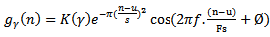(8)

Where dictionary D is then a set of elementary waveforms (sine modulated Gaussian functions) that can be generated by varying different parameters of , that are respectively: the frequency is used to quantify the frequency in (Hz) of the HFO burst. The time occurrence in (sample) is used to characterize the central timing of the HFO event. The scale (in sample) approximates the duration of the HFO pattern. The phase in (rad) corresponds to the phase of the HFO. Where is the sampling frequency. is chosen so that .

At the ith iteration (i =1..... M), a best-match atom is selected from dictionary D, which maximizes the correlation with the residual 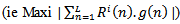. Where is the original signal and L its length. The procedure can be described by:

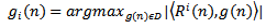(9)

Subsequently, the weighted best-match atom is derived from through the following equation:

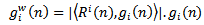(10)

And the next residual can be obtained by subtracting from the previous residual

(11)

In our previous studies, we used as an input parameter for training our algorithm an energetic parameter ().

represents the energy percentage of the synthesized signal compared to the input original signal. The synthesized signal is the sum of the extracted weighted Gabor atoms. Definition of the parameter is according to the following equation:

(12)

Where is the original signal.

A given signal cannot be perfectly synthesized by few atoms. Too few atoms (low value) could miss some true oscillations have low amplitudes (for example a Fast Ripple pattern), while too many atoms (high value) will end up in the last iterations as correction atoms (come from jumps, vertex waves, sharp waves, linearity…etc) which can be misclassified as true HFOs. In the fact, the main limitation for using parameter as an input setting for training our MP algorithm, that in last iterations when HFOs bursts have low amplitudes and low energies are going to be extracted by MP decomposition, the noise can be modeled by lengthy Gabor atoms have low amplitudes and significant energies. Therefore, noise has the priority to be modeled as spurious HFOs events compared to numerous relevant HFOs have both low energies and amplitudes together. That could increase the false detection rate. Thus, P parameter should be diminished, which would also decrease the sensitivity.

Another robust criterion was chosen for the detection of HFOs using MP, is to fit the signal in the first step with a high value of energetic parameter (P=99.99%), so that all relevant HFOs events can be extracted. Subsequently, a filtering MP in HFO band (80-500Hz) is applied. Each putative Gabor atom in the HFO band must satisfy the two following conditions to be as a candidate HFO: its amplitude (represents the input setting in the current study) must exceed a fixed threshold (its amplitude > and its scale must also exceed a duration threshold which is equal to . Where f is the assessed frequency of the considered Gabor atom, is the sampling frequency and c is the number of wave cycles is set to 3. Finally, as a final step, the grouping of overlapped detected Ripples and Fast Ripples into a single HFO event is done.

3.3. Detection of HFOs Based on Bumps Modelling Thechnique (BMT)

The bump modeling of a time-frequency map aims at representing the map with a set of predefined elementary parameterized functions called bumps[22]. The purpose of this technique was to reduce the huge quantity of parameters (hundreds of thousands coefficients) that describe a time-frequency map to a sum of parametric functions. A parsimonious representation is then obtained, which is relevant for further analysis, investigation and automated detection. The method is somewhat similar in spirit to the matching-pursuit algorithm that applied directly to the input original signal. In previous investigations, Bumps technique was successfully provides a quantitative estimate of the reproducibility of the time-frequency events[22]. Afterwards, it was used to investigate several aspects of brain oscillatory dynamics of Alzheimer's disease (AD)[22]. Bumps modeling technique was previously used for detection of HFOs bursts in[23]. Different details and improvement for detection of HFOs based on this method are described below:

3.3.1. Choice of Bump Function

Different kinds of functions were used for bump modeling. The prominent function that was used in the processing of EEG signals and led to a smaller modeling error is the half-ellipsoid function which is defined as follows:

(13)

Where

and are the coordinates of the center of the half-ellipsoid function. and are the half-lengths of the principal axes along the frequency and time axes respectively, and is its amplitude.

3.3.2. Resolution and Windowing

The time extension of wavelets is frequency-dependent: for high frequency, wavelets have a small time extension (high time resolution), but their frequency spectrum is large (low frequency resolution). Whereas, the inverse occurs at low frequency. The trade-off between the time resolution and frequency resolution is depending on Heisenberg-Gabor equation which is defined as follows:

(14)

Thus, time-frequency patterns to be modeled are characterized by a frequency-dependent time resolution as shown in equation.3. HFO seem as a sinusoidal signal that lasts at least 3 periods. Sliding windows defined as follows were used for modeling of the HFOs events:

- The time extension L (in sample) of a window centered at frequency f is equal to the duration of an oscillation. L is defined as follows:

(15)

Where Fs is the sampling frequency and N is set to 3 cycles.

Therefore, the ratio of the time extension L of the window to the time resolution of a wavelet at that frequency is defined as:

(16)

- The ratio of the frequency extension H of that window to the frequency resolution of the wavelet is also equal to 8π/7.

(17)

(18)

3.3.3. Define the Boundaries of the Map

For each point of the map under consideration, a time-frequency window centered at that point is obtained. Due to boundaries effect in time-frequency map, the section of signal to be modeled must start with a fixed duration equal to (Fs.(N/2*fl)) before the useful part of the signal and stopped after it with the same duration. The lowest frequency must be started with frequency and the highest frequency must be stopped at where is set to 400 Hz and is set to 80 Hz.

3.3.4. Search for the Zone Containing the Maximal Amount of Oscillatory Activity

The intensities map of the pixels contained in a window W describe the amount of oscillatory activity within the considered window. The modeling algorithm searches for the window Wmax containing the maximal energy amount: for each window W, the sum S of the intensities of the pixels within the window W is computed as follow:

(19)

The summation runs on all points within window W. The window Wmax with maximal S is then selected.

3.3.5. Bump Adaptation

Within the selected window Wmax, a bump function is adapted, starting with a bump extending over the whole area of the window. Thus, the bump function has five parameters, subject to the following constraints:

- are represent the center of the bump lies within the window Wmax.

- where L and H are the height and width of the window Wmax as defined by equation.15 and equation.18.

- Amplitude a > 0.

The adaptation phase is performed across the cost function E to be optimized based on the modeling error of the bump, defined by the sum of squared errors. The cost function is defined as follows:

(20)

Where the summation runs on all pixels within the window under consideration for instance.

When the bump is finally adapted, it is subtracted from the original time-frequency map, and the process is iterated with the next bump. The procedure of bumps decomposition is done across Butlf toolbox[24,25] decomposition available at:

http://www.bsp.brain.riken.jp/~fvialatte/bumptoolbox/toolbox_home.

Thus, each modeled bump is restricted to one biologically HFO oscillation with duration of three periods. Longer oscillations will be modeled by two bumps or more (non-overlapping or overlapping).

3.3.6. Termination Criterion

A trade-off usually exists between the rate of correct and false detection. If the number of bumps in the model is too low, the latter will not be sensitive; if it is too large, the noise will be modeled, hence irrelevant information would be built into the model, which could increase false detection rate. For the actual application, we first design a model with a largest number of bumps within a reasonable computation time (chosen header.limit parameter=0.0001[24,25]).

Subsequently, each extracted bump must satisfy the following conditions to be as a candidate HFO: its frequency must be included in HFO band (80-400Hz), and its fraction ratio F is defined in equation.21 should exceed a threshold (Fc). Fc is considered as the input parameter for training the current method (if F>Fc, Bump is considered as a candidate HFO, else is rejected). The fraction ratio (F) of the intensity modeled by a one given bump to the total intensity of the map is computed as follows:

(21)

The mentioned threshold (Fc) can also lead to a modified trade-off between the detected relevant HFOs and the detected spurious energetic oscillations come from the filtering of spikes without HFOs, sharp waves without HFOs, and backgrounds activities.

As a last step for HFOs detection using Bumps modeling, the grouping of overlapped detected Ripples and Fast Ripples into a single HFO event is then done.

4. Visual Marking of HFOs

Based on our custom Graphical User Interface (GUI), two reviewers trained in electrophysiology and HFOs analysis identified visually and independently all relevant HFOs included in the used channels. The visual marking of HFOs was performed by splitting the screen horizontally in which the reviewer can viewed a raw of unfiltered EEG and a filtered version (band-pass filtered at 80-500Hz) simultaneously. The unfiltered EEG signal is seen in the top plot and the filtered signal in the bottom plot. The filtered EEG is viewed at a higher gain than unfiltered EEG. The filter removes lower frequency components and helps to locate HFO events. The higher gain is necessary because HFOs have very low amplitudes compared to the unfiltered EEG signals. Each event is marked as a relevant HFO, if it seems as regular oscillation that has at least 3 consecutive periods, and can be clearly distinguished from the background activity in the filtered signal, and is confirmed in the unfiltered EEG signal. Each event detected by the two reviewers was considered as relevant HFO burst. The remaining events were excluded from the analysis. Finally, marked HFOs events were automatically saved in a database for future analysis.

5. Performance Metrics

Performance measure was quantified using the False Discovery Rate (FDR) which is a robust metric that characterize the false detection rate. The sensitivity metric is used to quantify the rate of correct detection. The two metrics are defined as follows:

(22)

(23)

HFOs detection software produces a list of candidate HFOs with their location, duration, and frequency. Candidate HFOs could overlap with Positives, Negatives. Positives: are different HFOs segments visually identified. Negatives: are different baseline segments. Pos: is the total number of positives. Dpos (Detected Positives): is the number of positives which overlap with at least one candidate-HFO. TP (True Positives): is the number of candidate-HFOs which overlap with at least one Positive event. FP (False Positives): is the number ofcandidate-HFOs which could not overlap with any positive event.

6. Result and Discussion

Previous studies[5,6] proved that visual marking of HFOs provides a good understanding of some underlying brain mechanisms for epilepsy. However, this visual process is highly time consuming, subjective and might be subject to error-prone. Fast, objective, reliable and automated detection of HFOs is necessary for the systematic investigation of HFOs and to propel the clinical use of them as a reliable biomarker of epileptogenic tissue. Another important benefit of automated detection process: permits to parameterize the detected discharges such as determination of their position, duration, amplitude and frequency, estimation of HFOs rates, and assessment of HFOs power. These extracted parameters may be very useful for investigation of important clinical information like the determination of underlying dynamic change of HFOs during inter-ictal[5,6,10], pre-ictal and ictal[9] periods.

Performance measure of HFOs detector depends on experts visual review- is considered the gold standard and must be associated with high inter-rater reliability. In the present study, 361 HFOs events were visually reviewed and considered as ground-truths for the performance measure and the comparison of the three improved existing HFOs detectors. The used data contains different background noise level, and includes both channels with active and rare HFOs rates. Receiver operating characteristic curves (ROC) of sensitivity vs. FDR, were used to test results of methods according to the different input parameters . 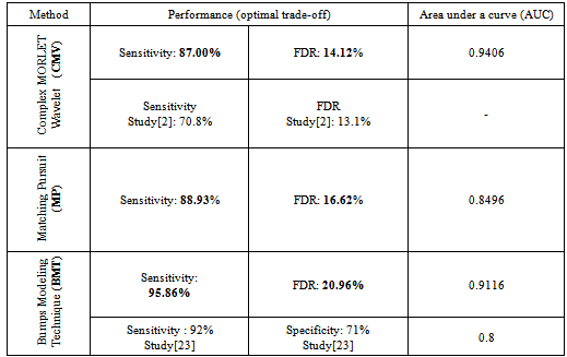The input parameters are respectively: the power threshold for CMOR wavelet based method, the amplitude threshold of Gabor atoms for MP method and the fraction ratio threshold for Bumps method. During the training, the varying input parameter was considered optimal when the discrimination between undesirable (spurious HFOs) and desirable events (detected positives) was maximized as much as possible. That means the difference between the sensitivity and the FDR should be maximized. The choice of this criterion is clearly justified by Rahul et al[2].

As is shown in figure.1, the optimal tradeoff between the sensitivity and the FDR for each method is indicated by the proper dash arrow for each curve. The table.1 illustrates a summarization of different results of the performance measure. The comparison is also done between our results and previous studies. Trapezoidal numerical integration method was used to determine the area under the ROC curves (AUC), the obtained AUC were respectively: 0.9406, 0.8496 and 0.9116.

Table 1. Summary of detection performance for different Methods

Figure 1. ROC curves of different methods: Optimal performance (best tradeoff) is indicated by the proper dash arrow for each curve

The main findings of the present study are summarized as follows: The efficiency of methods depends on the required sensitivity and FDR. First, If the required sensitivity below 87% is sufficient for the considered application, CMOR wavelet method could perform well in terms of low false detection rate (FDR<14%). Secondly, if the application requires a sensitivity between 87% and 92%, the three methods could perform in a similar way in terms of performance, which approximately corresponds to an FDR in the range of 14-19%. Finally, if a very high sensitivity is required (92% up to 98%), bumps modeling method can be considered the most efficient and can lead to significantly lower FDR values (19% to 23%) compared to other methods.

A snapshot of HFOs detection using CMOR wavelet (CMV) is illustrated in figure.2. The first plot represents the original EEG signal which is an active EEG segment. The second plot shows its corresponding time frequency map computed using CMOR2-1.114 wavelet family. Finally, automatically detected HFOs events are classified into true (relevant) HFOs events are indicated by the green rectangles and spurious detected oscillations are indicated by the red rectangles.

Figure 2. A snapshot of HFOs detection using CMOR wavelet. Optimal configuration for the power threshold: K1=2.1

A snapshot of HFOs detection using Matching Pursuit (MP) is illustrated in figure.3. The first plot represents the original EEG signal. The second plot shows the filtering of signal in the HFOs band. Finally, automatically detected HFOs events are classified into relevant HFOs events are indicated by the green rectangles and spurious oscillations are indicated by the red rectangles.

Figure 3. A snapshot of HFOs detection using Matching pursuit. Optimal configuration for the amplitude threshold of Gabor atoms: =5µv

A snapshot of HFOs detection using Bumps modeling technique (BMT) is illustrated in figure.4. The first plot represents the same original EEG signal. The second plot shows the time frequency map computed using CMOR 2.0558-0.5874 wavelet family. The third plot shows the extracted Bumps as candidate HFOs. Finally, automatically detected HFOs events are classified into relevant HFOs events are indicated by the yellow rectangles and false oscillations are indicated by the red rectangles.

Figure 4. A snapshot of HFOs detection using Bumps modeling technique. Optimal configuration for the Fraction ratio threshold is set to: Fc =0.00003

Different mentioned methods in the present study have advantages and disadvantages:

CMOR wavelet method is sensitive to detect HFOs, and good in terms of AUC. It might classify directly candidates HFOs into ripples and fast ripples. Moreover, it is faster than other methods. However, the fundamental limitation for this method is that most spikes and sharp waves without HFOs included in EEG recordings are better approximated as triangular pulses. The spectrum of triangular pulse is a squared-sinc function. Spurious blobs can be easily detected as probable HFOs come from side-lobe peaks of the squared sinc function.

Matching pursuit algorithm has also a good sensitivity. Moreover, the classification of candidate HFOs into ripples and fast ripples using the frequency of Gabor atoms can be done. The main limitation is that a given signal cannot be perfectly synthesized by few atoms. The extraction of all HFOs events using MP decomposition require model with high energetic parameter. In fact, high P value can cause a generation of correction atoms which essentially arising from reconstruction of jumps, vertex waves, sharp waves, linearity…etc. Correction atoms could have similar energies and amplitudes compared to numerous HFOs events. As result, using amplitude of Gabor atom as input setting can lead to a tradeoff between true and false detection, which usually cannot be avoided. In addition, it is possible that distortions may be generated by the subtractive step of MP. Long time computation is also considered as disadvantage for this method.

Bumps modeling based method is highly sensitive; the sensitivity could exceed 98% with a minimum FDR. It might classify directly candidate HFOs into ripples and fast ripples. Using CMOR wavelet decomposition as a first step of this method can produce several spurious blobs having significant energy in time frequency map. The mentioned spurious patterns come essentially from side-lobe peaks of the squared sinc function resulting from filtering of spikes and sharp waves without HFOs. Time consuming also considered as disadvantage for this method.

7. Conclusions and Perspectives

An automated and reliable detector is crucial for the investigation of HFOs and for the understanding of their relationship to the underlying pathology in epilepsy.

Thus, several automatic detectors were developed for different EEG recordings and with different aims. Improving and comparing them in a single dataset is important to analyze their performance and robustness. The efficiency of the tested methods described in the current study depends on the required sensitivity and the FDR, which are related to the intended application (supervised or unsupervised detection method, time computation, complexity,…).

As a conclusion, the three algorithms described here can achieve a high sensitivity. Bumps modeling based method can achieve a high sensitivity up to 98% with the minimum FDR compared to MP and CMOR wavelet based methods.

To date, there can be an overlap between the time–frequency representation of transients (spikes, sharp waves, artifacts) and HFOs oscillations. The majority of HFOs detection methods are frequency based decomposition that can lead easily to detection of false-positive events, which arise essentially from the filtering of spikes and sharp waves without HFOs. Still, the best method must have as much sensitivity as possible to correctly detect all true HFOs events included in EEG data. False detection should be reduced to the minimum as possible. Also the best method should not be sensitive to spikes/ sharp waves without HFOs. In addition, such a robust detector should perform in a similar way for all types of channels with active and rare events and for different background levels.

Further studies based on advanced signals processing are needed, such as the approaches based on mathematical morphology and geometric analysis, which may discriminate between transients without HFOs and transients with HFOs. This can improve the detection performance of different algorithms in large scale. Another potential interesting path that could be further explored is to address the question of whether a consensus automatic procedure that combines all three available methods (e.g. letting each method vote on each event) could outperform the results of a single approach. This can also improve our results and reduce false detection rate. Still, fast software and powerful systems are needed. Our future work will be focused on analyzing large amounts of EEG data using scalp EEG recordings and Invasive EEG based on a consensus automatic procedure that combines all the three available methods.

ACKNOWLEDGEMENTS

Authors wish to thank the Montreal Neurological Institute and Hospital (MNI, Canada) for kindly providing database which we used to test and compare the performance of current methods. We would like to thank Dr. Mohamed Dogui (Service of Functional Exploration of the Nervous System, CHU Sahloul of Sousse, Tunisia) for helping us doing visual identification process of high frequency oscillations in EEG.