1. Introduction

A fundamental problem in remote sensing discipline, as well as in many other applications (biomedical signals, telecommunication, etc…), is to find a suitable representation of multivariate-observed data to extract the useful information within the observed data[1]. Given that, this information is subject of several perturbations, it is in general, not directly accessible. The main aims of this work are; firstly, to identify the transfer function of linking signals of interest (sources) to the observations, and secondly to restore the valuable information[2]. To overcome these problems, we develop an approach based on the Blind Source Separation (BSS) which describes techniques that aim at separating signals if no information is available about the original sources[3]. This technique is an important field of research in signal and image processing. It was introduced and formulated by Bernard Ans, Jeanny Herault and Christian Jutten[4, 5] since the 80’s, and it raises now great interest. This situation is common to communication signals[6, 7], biomedical signals[8, 9] and astrophysical data analysis[10, 11]. Recently, this technique is adapted to remote sensing (multispectral and hyperspectral imaging) to obtain more accurate representation of the geological and vegetative ground surfaces[12, 13]. In fact, the large dimension of hyperspectral images needs and the heterogeneity of ground surfaces need to use various methods to describe image features.

In order to solve the problem of source separation, we seek to maximize the statistical independence between the different components of the estimated sources. An alternative approach to the BSS problem is to assume that the sources have a sparse expansion with respect to some basis (or dictionary)[14]. Briefly, a signal is said to be sparse according to a given basis if most of his entries (or elements) have no significant amplitudes. To take advantage of hyperspectral images, we propose to explore a novel approach based on source separation in a frequency-domain. Thus, independence and sparsity which are the main hypotheses of all the source separation techniques are not required for the source images themselves, but rather for their spectra[14, 15]. The proposed approach has the added advantages of the DCT and second-order statistics. The first exploits the inter-pixel correlation and the second exploits the inter-band redundancies. Both theoretical and algorithmic comparisons between separation in the spatial and DCT-domain are given. Thus, we associate statistical methods of BSS to different classification techniques to achieve a better result for the classification of hyperspectral data. This work is reached by employing Second-Order Separation by Frequency-Decomposition. Termed SOSFD, this technique uses joint information from second-order statistics and sparseness decomposition. In this regard, this paper is organized as follows: First, we present a formulation of the problem of BSS and we clarify the related theoretical elements. Second, we establish the frequency-based approach on hyperspectral data. Finally, we study the results to show the contribution of this new approach on hyperspectral images and we prove the performance of the SOSFD algorithm.

2. Background

2.1. Source Separation Principle

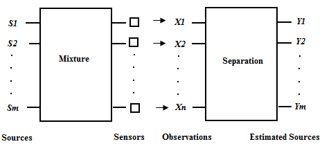
The source separation method can be applied to hyperspectral imaging to separate the components and make them statistically independent. This method is the most appropriate for our study, since the observation images show a strong correlation between them. The principle of source separation technique consists in the extraction of unknown source signals from their instantaneous linear mixtures by using a minimum of prior information: The mixture should be “blindly” processed[7, 16-18]. So, we describe this technique from m random processes or observations, noted {x[k]} _kϵN=[x₁[k]…x_m[k]]^T that result from a linear mixture of n random processes or sources, noted {s[k]} (s[k] =[s₁[k]…s_n[k]]^T). The general configuration of sources separation is shown in Figure 1.

Figure 1. General configuration of source separation

In recent years, great part researches work in BSS relevant source separation assuming a linear mixing application A. For a linear mixing convolution MIMO (Multiple Input-Multiple Output) is described in the following equation:

(1)

(2)

where x[k] is a m×T noisy instantaneous observed signals, s[k] is a n×T source signals, (b[k] =[b₁[k]…b_m[k]]^T) is a m×T additive noise corrupting the observation images and A is a m×n mixing application. BSS technique consists of finding an application G known as a separator, such that: y[k]=G(x[k]). Furthermore, the separator G is an n×m matrix and y[k] is an estimate of s[k] to a trivial matrix of the form Λ ∏ which Λ and ∏ are respectively diagonal and permutation matrix, such that:

(3)

To ensure that the problem of BSS is well posed, the hypothesis that is generally accepted is that the sources s[k] _keN, are statistically independents[20-24]. The realism of this assumption in a number of real-world problems is obviously fully justified. But, a difficulty arises when the mixing matrix A is unknown, so how can we invert a matrix that is unknown? That it leads to determining Â^-1, an estimate of the inverse of the mixing matrix A^-1. Observations will be transferred to the system that performs Â^-1 to infer an estimate of the sources (Figure 2). This gives:

(4)

Figure 2. Classical approach for linear mixing

In the BSS approach, the instantaneous linear mixing hypothesis has and continues to stimulate a great interest, both in terms of application and methodology[2]. Nowadays, we have number of BSS tools which prove performers in theory, but it remains to study their behaviour in practical situations such as in remote sensing domain[25, 26]. Therefore we emphasize, in this work, on the method of source separation using second-order statistics for hyperspectral images to obtain more accurate representation of the ground surfaces.

2.2. Source Separation Methods

In the beginning of 80s, research in the domain of BSS has been initiated by Bernard Ans, Jeanny Hérault and Christian Jutten in the modelling of decoding movement in vertebrate’s problem. The authors proposed an approach to separate sources based on neural networks[27, 28]. Since this work, many BSS algorithms have been developed[4, 5]. We will present, in this section, some methods of blind source separation such as SOBI, JADE and fastICA.

• SOBI (Second-Order Blind Identification, Belouchrani and al. 1997) exploits not one but several covariance matrices of the observations. The authors show that after whitening observations, a joint diagonalization criterion was used to estimate the mixing matrix[18].

• JADE (Joint Approximate Diagonalization of Eigen-matrices, Cardoso and Souloumiac 1993) presents an algebraic solution to the maximization of contrast based on the fourth order cumulants[29-31].

• FastICA (Fast Independent Component Analysis, Hyvärinen and Oja 1997) exploits the principle of neguentropy approximated by the absolute value of kurtosis of the estimated sources[32, 33].

Hyperspectral data[34-36] can be modelled in the form of instantaneous physical mixtures. The required sources have a physical origin and their mixing coefficients are the unknown proportions. The intrinsic content of the sources is temporally or spatially correlated, moreover the mixtures exhibit localized spectral information. This description affects the choice of the algorithm.

Therefore, one can use the second-order statistics which consider the spatial or temporal correlation[18, 37], by applying the following SOBI algorithm which is well adapted to this situation and provides robust solution for sources separation. In addition, data such as hyperspectral images suggested further development derived from SOBI with mixing the second-order statistics and an orthogonal inverse transformation like DCT. This study will be largely explained in the following sections.

3. Second-Order Separation Approach

The Second-Order Blind Identification (SOBI) is one of the well known second-order based approach to calculate the separating matrix. Therefore, we can assert that the separation is complete when the estimated sources are as spatially independent as possible. Accordingly, the separation task is achieved in two steps; the first step consists of whitening the signal of observation by applying a whitening matrix. The second step is to apply the joint diagonalization of several covariance matrices of whitened signal vector[20, 37-40].

3.1. Whitening

This step consists of “whitening” the observed signal x[n]. This is achieved by multiplying x[n] by an n×m whitening matrix W which satisfies

(5)

where H denotes the conjugate transpose and R_S(0)=I.

Being a linear transformation, the whitening step is performed to decorrelate and enforce a unit variance of variables of the vector x[n]. Consequently, through the whitening procedure, we only need to estimate the unitary mixing matrix WA=U, with U is an n×n matrix instead of estimating an m×n mixing matrix parameters. The matrix A can be taken as

(6)

So

(7)

where, # denotes the moore-penrose pseudo-inverse.

3.2. Joint Diagonalization

The whitening operation as described in the previous section consists in finding an affine transformation that associate to x[k] a vector process whose covariance matrix is identity. Therefore, the new system (z (t)) guarantees a unitary mixing matrix as follow

(8)

And W can be estimated from the covariance matrix of the signal x (initial process). In fact, the covariance matrix is diagonalizable by U, and certifying its existence:

(9)

where ρ_i(τ)=E[S_i(t+τ)S_i^*(τ)] is the auto-covariance of s_i and diag[.] is the diagonal matrix formed by the elements of its argument. Thereafter, the question is how we can find the matrix U from the diagonalization of the covariance of the whitened process at a given delay τ ?

The favourable solution that overcomes this problem is equivalent to diagonalizing jointly several covariance matrices with several delays which increases the robustness of the separation. Then the estimate of the sources will be possible after the estimation of the matrix U.

In this manner, the source separation technique using second-order statistics is achieved using statistical information available on sources at any time lag.

4. Sparsity Representation

Recently, the sparse representation of signals and images is a problem that has been drawing considerable attention and widely studied in many recent applications like in remote sensing. In this paper, we propose a novel structure of such a database for representing image content in order to select the optimum data information. In fact, representing the hyperspectral images in well suited database functions allows a good distinction of various types of objects. In this paper, we apply a new source separation algorithm which is based on sparse representation of real hyperspectral data and show that choosing an appropriate basis is a key step towards a good sparse decomposition to improve the hyperspectral data analysis[14, 41]. So, we explore in this work the sparse decomposition of hyperspectral data by using DCT and we will explore the effect of sparse basis on dataset. Using the sparseness assumption, the following method illustrates the use of the mixing structure in order to estimate the mixing matrix[42-44].

We will define the model of sparse representation with a more formal way. Assuming a signal x is a vector in a subspace of finite dimension x=[x[1],…, x[N]]. x is accurately sparse if most of its components are zero, i.e. its support supp(x)={i/ 1 ≤ i ≤ N and x[i]≠0} become, if sparse, |supp(x) |=K << N and the signal x is said K-sparse. In most applications, the signal is sparse in an appropriate transformed domain but not in its original one, so x can be written in a suited basis D as follows:

(10)

where supp(α)=K << N and α[i] is the coefficient representing the contribution of the atom φ_i of the dictionary D in x.

To estimate the sources, it is sufficient to find a representation in the form of a set of coefficients S such that s = SD where S is an unknown sparse matrix. In order to simplify the problem, BSS method based on sparsity exploits the matrix S that contains few coefficients significantly different from zero[45-47]. By combining the representation s = SD with the instantaneous mixing model x = As, we find:

(11)

The objective of BSS in the transform domain is to compute a new representation x=XD with X=AS following the structure of the chosen dictionary[47, 48].

5. Data and Processing Methods

5.1. Data Description and Methodology

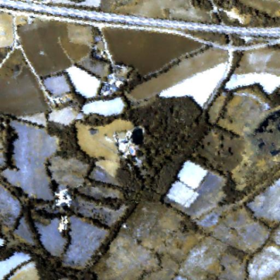
Figure 3. CASI composite image of three colours (RGB)

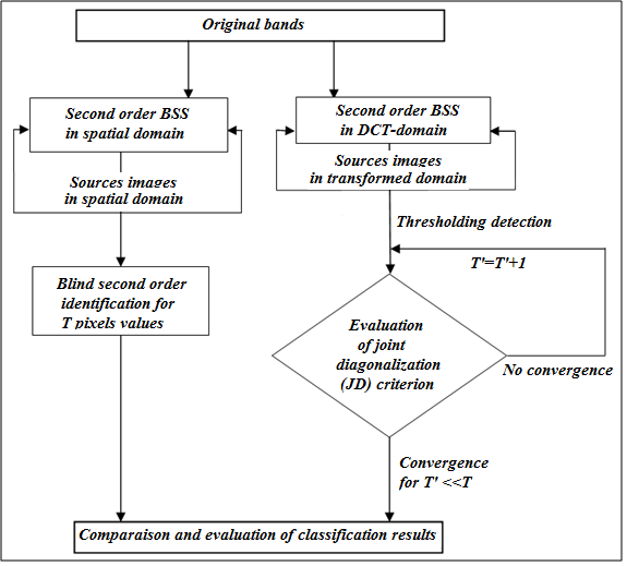
Figure 4. Methodology

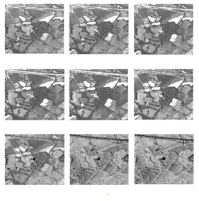
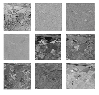
Figure 5. CASI image in the 9 spectral bands

In this work, we use the Compact Airborne Spectrographic Imager (CASI) data (Figure 3). The number of bands collected by CASI can be so great. This sensor can acquire up to 228 spectral bands between the wavelengths 400 to 1000 nanometres[49]. The proposed method described in Figure 4, shows a methodology based on two source separation techniques to evaluate hyperspectral classification: The first is in special domain and the second in a transformed domain. The latter shows a good performance and should minimize the misclassification risk of dataset.

To describe the source separation approach and to illustrate the corresponding results, we will use 9 observation images extracted from the CASI sensor, between the wavelengths 551.1 to 799.9 nanometres, by experts as the most pertinent to increase the reliability of the analysis of the study zone (Figure 5).

5.1. Processing Methods

5.1.1. Classical Source Separation

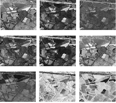
Figure 6. Sources in image-domain

The source separation method produces source images represented according to mutually independent axes. Therefore, there is a decrease in the rate of correlation between the source images. At this level, the decorrelation is achieved in the spatial-domain by the SOBI (Second-Order Blind Identification) algorithm[13, 51]. Thus, a visual analysis shows the important contribution of the source separation method to discriminate natural themes compared to original images (Figure 6). However, some sources don’t have a physical sense and we cannot identify for them a significant theme like source 2, source 3 and source 4.

5.1.2. DCT-Domain Separation

To provide a valid decomposition of the hyperspectral images, we adopt a blind and automated procedure that relies on an optimal decomposition of the image spectra. The frequency approach used in this work is implemented by mixing DCT and second-order statistics. Since DCT is a linear orthogonal transformation, it can be applied either on spatial or on spectral data[52]. The used criterion should provide independent information turned to distinct spectra. The extracted independent components may lead to a meaningful data representation which permits to extract information at a finer level of precision[53]. The positive effect of such transformation is the removal of redundancy between neighbouring pixels in the first stage and the discrimination between low and high frequency of bands in the second stage.

In this paper, we use the source separation criterion in the frequency-domain[46, 54]. Therefore, the particularity of SOSFD approach is to implement the DCT in order to extract independent spatial-frequency sources. The DCT exploits inter-pixel redundancies to turn into excellent decorrelation for most natural images. The frequency source separation method can be modelled by the following form

(12)

Hence, the source separation problem is transformed to the DCT-domain. The superscript (T) indicates that the related matrix is of T columns. Furthermore, DCT exhibits excellent energy compaction for highly correlated images such as hyperspectral images and because the noise produces DCT-coefficients that are close to zero at a smaller frequency, we can model our frequency-based approach by a free noisy form

(13)

where X_dct ^(T’) is a m×T’ matrix and S_dct ^(T’) is a n×T’ matrix with (T’) << (T). (T’) is chosen to give the most important coefficients. So, T' corresponds to coefficients with the largest energy of the transformed images. The separation complexity can be reduced by manipulating (T’) DCT-coefficients instead of (T) pixel values.

Then, to ensure the identification of the sources and to improve the statistical efficiency, we estimate the dominant independent orientation from only the most significant DCT-coefficients (Figure 7). In fact, we adopt in our work an algorithm of independent component analysis in the frequency-domain.

Figure 7. Transformed domain 2D-DCT of hyperspectral image

5.1.3. Algorithm Implementation: SOSFD Algorithm

The frequency-separation criterion is based on the following steps:

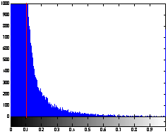
• Determining the threshold from the histogram obtained by computing K which is the mean of all coefficients of a homogeneous DCT basis

(14)

The normalized histogram defined in the set of {0, (T)-1} in[0, 1], present the proportion of samples in K. So, we can set the number of iteration and the threshold (T’). The operation (T’)=(T’)+1) is recursively until convergence (Figure 4).

• Reducing the number of parameters to be estimated by whitening the observed process X_dct ^(T). So, the step of whitening is based on the covariance matrix and it is done by eigenvalue decomposition which is equivalent to Principal Components Analysis (PCA). This process consists of whitening X_dct ^(T), the signal of observation by applying a whitening matrix W.

(15)

The whitened process Z_dct ^(T) still obeys a linear model given by

(16)

where U is a n×n unitary matrix. Hence, instead of estimating the m×n mixing matrix parameters, we only need to estimate the unitary mixing matrix which contains only n×(n-1)/2 degrees of freedom

• Determining the unitary factor U from a unitary diagonalization of a whitened covariance matrix R_dct (ν) for any frequency shift ν ≠ 0.

(17)

where D is a diagonal matrix.

• The existence of a frequency shiftν, such that R_Zdct (ν) yields the relevant parameters, is directly linked to the existence of distinct eigenvalues of R_Zdct (ν). To increase the statistical efficiency of the estimation, we can consider a joint diagonalization of several covariance matrices R_Zdct (ν_i)1<i<n for n different frequency shifts (ν_i)1<i<n. From the spectral theorem, we can jointly diagonalize the set of covariance matrices by a unitary matrix V that is essentially equal to U[19]. This leads to minimize the following joint diagonality (Jd) criterion.

(18)

Then the source coefficients in the DCT-domain are estimated as is styled.

(19)

And then, by the inverse DCT-transform, we determine an estimate of the source matrix Ŝ and an estimate  of the mixing matrix A such as

(20)

6. Experimental Results and Evaluations

First, we illustrate the benefit of the blind source separation in the DCT-domain by comparing the performance of SOSFD approach with the classical second-order source separation that performs in the spatial-domain[18].

6.1. Joint Diagonalization Performance

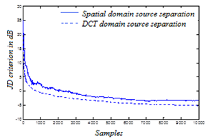
The performance measure used to judge the quality of the separation is the Joint Diagonalization (JD) criterion defined by the relation (18). In Figure 8, the JD criterion is plotted in decibels against sample size. The DCT-domain curve shows a performance gain reaching 5dB compared to the image domain curve. A sketch of the proof of the efficiency of the Joint diagonality criterion, when applied in the DCT-domain rather than in the original spatial-domain, is given in following section.

Figure 8. JD criterion evaluation

6.2. Power Spectral Density Evaluation

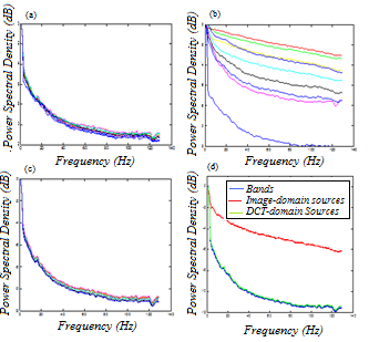
In this section, we illustrate the performance of our approach on hyperspectral data, which are known to be sparse in the DCT-domain. At the beginning, we consider the hyperspectral observations. Before processing, we show the power spectral density of these images (Figure 10-a). This figure illustrates the huge correlation between the power spectral densities of the hyperspectral images.

These spectral densities show a large number of spectral components with very weak amplitude. This reduces the calculus complexity when dealing with source separation in the DCT-domain.

In (Figure 10-b), the source power spectral densities look more separated using second-order statistics in the spatial-domain.

The data resulting from the new source separation approach are presented in Figure 9. We can note a more effective discrimination between the different classes. The later are represented more clearly by maximizing the contrast between them, which can improve the accuracy of the classification process.

Figure 9. Resulting data after source separation method

In fact, this new approach produces source images represented according to independent axes that will therefore permit an important decrease of the correlation between the extracted sources and allow a more efficient representation of information contained in each image. Then, each source can represent specifically certain themes. Let us note that the DCT is a linear transform that is used to represent the frequency-content of image data in terms of amplitude or energy. This transformation is studied to establish the link between the frequency-distribution and structural composition of the image. The decomposition of data by the DCT employs information contours of low frequency, midrange and high frequencies to energy at the edges. Consequently in comparison to Figure 10-a, the sources resulting from the new approach (Figure 10-c) are physically more meaningful; they maintain the spectral properties of the data while gaining the edge information.

The effect of our approach is also seen from the power spectral densities of the DCT-components. The corresponding sources are then identified reliably due to the distinct differences in their power spectra.

It is interesting to note that the most important spectral components of the new sources (Figure 10-d) are accumulated in the same frequency-range 0-15 Hz of original images (Figure 10-a); as opposed to the power spectra of the spatial-domain sources (Figure 10-b), which are ranging in a larger frequency-domain. This figure describes the source energy distributions according to the frequency-domain.

Figure 10. Power spectral density of (a) the observation components, (b) the spatial-domain sources components, (c) the DCT-domain source components and (d) The mean power spectra of the original bands, spatial-domain sources and DCT-domain sources

Classical BSS is a mathematical or statistical method, so that the physical sense of BSS is not obvious. We are simply attempting to make the estimated sources independent. Subsequently, the DCT-decomposition of images provides a physical understanding of frequency-domain BSS.

When applied in the DCT-domain, second-order statistics permit to group and separate the different spectra around each dominant frequency. This permits to give a physical sense to each generated source. The result of Figure 10-d is in excellent agreement with the previous results. The mean power spectrum of the DCT-domain source is in correlation with the mean power spectra of the original bands which enhances the physical interpretability of these sources (Figure 10-d). However, the mean power spectral of the sources in spatial domain (Figure 10-d) is spreading in a larger frequency-field particularly in the high frequency-field. Indeed, even if the hyperspectral data does not physically verify the independence test, BSS can find directions in which the components are independent. The estimated directions are less Gaussian thus most asymmetric, which can improve the image classification. In fact, the BSS as mathematical approach better characterizes the relationship between components that are actually almost non-orthogonal. The large high frequency-power spectral values don’t guarantee the physical interpretability; this led to three non significant extracted sources, like the source 2, 3 and 4 of the Figure 6.

6.3. Classification Method Evaluation

In order to evaluate the performance of the proposed approach, we use a traditional supervised method, which is the Maximum Likelihood (ML) classifier[55]. The ML classifier is a spectral parametric classifier that characterizes the pattern of each class in terms of its pdf, the form of which is assumed to be known in advance. The pdfs are usually multivariate Gaussian functions so the only need to estimate the mean vector and the covariance matrix. The estimation accuracy of the ML method is generally high. This method allows designing an optimal classifier to make available a statistical model which giving description of the observations xX and the hidden state cC. This statistical model must be estimated from the training set

(21)

with is the estimated distribution of conditional probability. The estimation of the joint probability is the goal of this step, according to the information existing in the training set. The observed data are given as

(22)

for supervised learning. The latter method is categorized on the use of the input and target samples in order to estimate a mapping from the input to the output based on a probabilistic model.

For the likelihood function, we use a parameterized density for modelling a set of data D. In assumption to be drawn independently from, the likelihood function can be modelled in the following form

(23)

Subsequently, we can find the most advantageous values for the parameters by estimating the ML function from the training data by maximizing the log-likelihood function

(24)

In fact, the ML finds a parameter available to best explaining the examples by

(25)

This can be obtained under finding the stationary points

(26)

Characterized by mean and covariance, the Gaussian distribution has simple analytical properties. It is needed to estimate two parameters θ₁ and θ₂ which are respectively the mean vector value and variance value

(27)

(28)

Before starting the discussion of results, we must define the terms for evaluating our results. Firstly, we identify the confusion matrix as error matrix which displays the degree of misclassification among classes. In fact, the quality of the classification is expressed by the number of pixels correctly identified in the total for the studied area. The confusion matrix is a square matrix of size equal to the number of classes and whose elements represent the number of well assigned pixels of each ground truth according to the corresponding classes. Among the indicators of relative accuracy, we cite the Omission Error (OE) and the Commission Error (CE) by

(29)

and

(30)

with X_ij, X_il and X_cj are respectively the elements of the confusion matrix, the sum of row elements and the sum of column elements of the confusion matrix. From there, a global measure representing the average rate of correct classification can be obtained such as the Kappa coefficient K

(31)

with N_P, M_c and X_Dii are respectively the total number of data pixels, the total number of existing classes and the diagonal elements of the confusion matrix. In this work, we used the classification Error Rate (ER) to test the performance of the classification. This indicator is obtained by

(32)

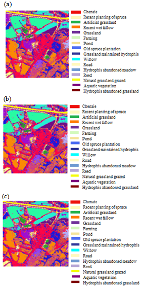
Figure 11 provides the classification result for initial bands (Figure 11-a), sources in the spatial-domain (Figure 11-b) and sources in the DCT-domain (Figure 11-c). This classification was done using sixteen input classes identified from a ground truth chosen by experts who are familiar with the terrain.

The ER is of 14.54%, 12.14% and 11.97% respectively for the initial bands, the spatial-domain sources and DCT-domain sources.

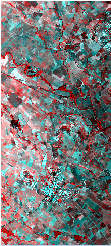
Then, the proposed approach is applied to other hyperspectral Mapper (Hymap) data (Figure 12). This sensor can acquire 126 spectral bands between the wavelengths 438 to 2483 nanometres[50]. Figure 13 provides the classification results for initial bands (Figure 13-a), sources in the spatial-domain (Figure 13-b) and sources in the DCT-domain (Figure 13-c). The ER is of 24.88%, 19.24% and 17.15% for the initial bands, the spatial-domain sources and DCT-domain sources respectively.

Figure 11. Classification results for (a) initial bands; ER=14.54%, (b) spatial-domain sources; ER=12.14% and (c) DCT-domain sources; ER=11.97%

Figure 12. Hymap composite image of three colours (RGB).

Figure 13. Classification results for (a) initial bands; ER=24.88%, (b) spatial-domain sources; ER=19.24% and (c) DCT-domain sources; ER=17.15%

These experiment results show that the sources generated in the DCT-domain present the lowest classification ER and can provide a reliable tool for hyperspectral image classification.

7. Conclusions

This study confirms the potential of the DCT-transform for some image-treatments. In this paper, we present a novel approach to separate hyperspectral data in the spectral-domain. Indeed, the hyperspectral images present a strong correlation which affects the extraction of significant information linked to ground truth. The joint application of the source separation method and the DCT-transform allows a more efficient representation of the spectral data and increase the reliability of the analysis of these images. The sources resulting from the new source separation approach are then identified reliably due to the distinct differences in their power spectra. The main conclusion to be drawn from this research study is that the application of the second-order source separation approach in the DCT-domain reduces the classification ER of the hyperspectral images. The use of a supervised classification shows that the sources generated in the DCT-domain present the lowest classification error and the more decorrelation between image themes. The ER is of 14.54%, 12.14% and 11.97% respectively for the initial bands, the spatial-domain sources and DCT-domain sources. By applying the SOSFD algorithm to another data set, the ER is of 24.88%, 19.24% and 17.15% for the initial bands, the spatial-domain sources and DCT-domain sources respectively.

To take advantage from the new representation of hyperspectral data, we propose a novel classification approach based on using Binary Partition Trees (BPT). The BPT is obtained by iteratively merging regions and provided a combined and hierarchical representation of the image in a tree structure of regions. The proposed strategy incorporates spatial information with spectral information by jointly using the adjacency information. Indeed, this methodology is based on the consideration of spatial attributes in the model and region merging criterion.

Appendix

In this section we prove the efficiency of the Joint diagonality criterion when applied in the DCT-domain rather than in the original spatial-domain.

The source separation problem in the DCT-domain consists of searching m × n matrix A, such that the S_dct^(T’) components are as independent as possible. Thus, the independence assumption is not required for the source signals S but for their DCT-coefficients, which is more plausible thanks to the sparse property of the DCT-coefficients. Thanks to the last property, most columns of S_dct^(T’) contain at most one significant term, so we have

(33)

with the number 1 at the l_th position.

The source covariance matrices in the spatial and DCT-domain, for any frequency shift ν_k, can take the following form

(34)

(35)

where D is composed from the diagonal elements of the covariance matrix and R=R(ν_k)-D.

Then, from (33) we can have the following inequality

(36)

Thanks to the diagonal structure of D, we can write

(37)

and

(38)

Because the inequality (38) is unchanged up to permutation and scalar factor, we can have for any k

(39)

where P is a permutation matrix and D is a diagonal matrix.

So that, there exists a unitary matrix V that is essentially equal to U such that

(40)

Then, we obtain

(41)

The form (41) proves the efficiency of the Joint diagonality criterion when applied in the DCT-domain rather than in the original spatial-domain.

References

[1]  Aapo Hyvärinen and Erkki Oja, “Independent Component Analysis: Algorithms and Applications”, Neural Networks Research Center, 13(4-5), 411-430, 2000.
[2]  Amar Kachenoura, Laurent Albera and Lotfi senhadji, “Séparation aveugle de sources en ingénierie biomédicale”, Article original, Science Direct ETSEVIER MASSON, ITBM-RBM 28, 20–34 (2007).
[3]  Ali Mansour, Kardec A Barros, and Noboru Ohniski, “Blind separation of sources: Methods, assumptions and applications”, IEICE Trans. Fundamentals Electron. Commun. Comput Sci., vol. E83-A, no. 8, pp. 1498–1512, Aug. 2000.
[4]  Pierre Comon, Christian Jutten, " Séparation de sources 1 : concepts de base et analyse en composantes indépendantes ", Ed. Lavoisier, Paris 2007.
[5]  Pierre Comon, Christian Jutten, " Séparation de sources 2 : Au-delà de l'aveugle et applications ", Ed. Lavoisier, paris 2007.
[6]  K. Anand, G. Mathew, and V. Reddy, “Blind separation of multiple co-channel BPSK signals arriving at antenna array,” IEEE Signal Proc. Lett., vol. 2, no. 9, pp. 176–178, Sep. 1995.
[7]  E. Chaumette, Pierre Comon, and D. Muller, “ICA-based technique for radiating sources estimation: Application to airport surveillance,” Proc. Inst. Electr. Eng.—F, vol. 140, no. 6, pp. 395–401, Dec. 1993.
[8]  Lieven De Lathauwer, Bart De Moor, and Joos Vandewalle, “Fetal electrocardiogram extraction by source subspace separation,” in Proc. HOS, Aiguablava, Spain, Jun. 1995, pp. 134–138.
[9]  Scott Makeig, Anthony J Bell, Tzyy P Jung and Terrence J Sejnowski, “Independent component analysis of electroencephalographic data,” in Advances in Neural Information Processing Systems, vol. 8. Cambridge, MA: MIT Press, 1995.
[10]  Albert Bijaoui and Danielle Nuzillard, “Blind source separation of multispectral astronomical images,” in Proc. MPA/ESO/MPE Joint Astronomy Conf., A. J. Banday, A. Zaroubi, and A. Bartelmann, Eds. Garching, Germany: Springer-Verlag, 2000, pp. 571–581. 31/7-4/8.
[11]  Danielle Nuzillard and Albert Bijaoui, “Multispectral analysis, mutual information and blind source separation,” in Proc. 2nd Symp. Phys. Signal and Image Process., 2000, pp. 93–98.
[12]  M. Lennon, G. Mercier, M. C. Mouchot, and L. Hubert-Moy, “Spectral unmixing of hyperspectral images with the independent component analysis and wavelet packets,” in Proc. IGARSS Conf., Sydney, Australia, Jul. 9–13, 2001.
[13]  Mohamed A Loghmari, Mohamed S Naceur and Mohamed R Boussema, “A spectral and spatial source separation of multispectral images”. IEEE Trans. Geosci. Remote Sens.,vol. 44, no. 12, pp. 3659-3673, Dec 2006.
[14]  Jérôme Bobin, Jean L Starck, Jalal M Fadili, and Yassir Moudden, “Sparsity and Morphological Diversity in Blind Source Separation”, IEEE Trans. on Image Processing, vol. 16, pp. 2662-2674, Nov. 2007.
[15]  Jérôme Bobin, Jean L Starck, Yassir Moudden, and Jalal M Fadili, “Blind source separation : The sparsity revolution”, In Peter Hawkes, editor, Advances in Imaging and Electron Physics, volume 152, pages 221–298. Academic Press, Elsevier, 2008.
[16]  I.Gorodnitsky and Adel Belouchrani. Joint Cumulant and Correlation Based Signal Separation with Application to EEG Data, Proc. 3-rd Int. Conf. on Independent Component Analysis and Signal Separation , I:475-80, (2001).
[17]  Jean F Cardoso, “Blind signal separation: statistical principles” Proceedings of the IEEE. Special issue on blind identification and estimation, vol. 9, no. 10, pp. 2009–2025, Oct. 1998.
[18]  Adel Belouchrani, K. Abed Meriam, J.-F Cardoso and E. Moulines, “A blind source separation technique using second-order statistics” IEEE Transactions on Signal Processing, vol. 45, no. 2, pp. 434-444. Feb. 1997.
[19]  M. S Pedersen, J. Larsen, U. Kjems, and L. C. Parra, “A survey of convolutive blind source separation methods”, Springer Handbook on Speech Processing and Speech Communication”, ISBN 978-3-540-49125-5, 2007.
[20]  R.R. Gharieb, and A. Cichocki, “Second-order statistics based blind source separation using a bank of subband filters”, Digital Signal Processing 13 252–274 (2003)
[21]  Aapo Hyvärinen, “Survey on independent component analysis”, Neural Comput. Surveys 2, 94–128, (1999).
[22]  Aapo Hyvärinen, “New approximations of differential entropy for independent component analysis and projection pursuit”, Adv. Neural Inform. Process. Systems 10, 273–279 (1998).
[23]  S. Amari, A. Cichocki, H.H. Yang, “A new learning algorithm for blind signal separation”, Adv. Neural Inform. Process. Systems 8, 752–763 (1995).
[24]  S. Choi, A. Cichocki, A. Beluochrani, “Second order non-stationary source separation”, J. VLSI Signal Process. 32 (1/2) 93–104 (2002).
[25]  Danielle Nuzillard and Albert Bijaoui, “Blind source separation and analysis of multispectral astronomical images”, Astron. Astrophys. Suppl. Ser. 147, 129{138 (2000).
[26]  J.Wang and C.I Chang, “Independent component analysis-based Dimensionality Reduction with Applications in Hyperspectral Image Analysis”, IEEE TRANSACTIONS ON GEOSCIENCE AND REMOTE SENSING, VOL. 44, NO. 6, JUNE 2006.
[27]  J. Herault, Christian Jutten and B. Ans, «Détection de grandeurs primitives dans un message composite par une architecture de calcul neuromimétique en apprentissage non supervisé ». In: GRETSI 85, Dixième colloque sur le Traitement du Signal et des Images, Nice, France. p. 1017–22. (1985)
[28]  Christian Jutten, J. Herault, “Blind separation of sources, part: an adaptative algorithm based on neuromimatic architecture”; Signal Process; 24 (1):1–10. (1991).
[29]  Y. Li, D. Powers and J. Peach, “Comparison of Blind Source Separation Algorithms”, Mastorakis, Advances in Neural Networks and Applications, WSES (2000) p18-21.
[30]  Jean F Cardoso, Antoine Souloumiac, “Blind beam forming for non-Gaussian signals”. IEE Proceedings-F: radar and signal processing; 140(6): 362–70 (1993).
[31]  J Jean F Cardoso , Antoine Souloumiac, “Jacobi angles for simultaneous diagonalization”; SIAM J Matrix Anal Appl; 17(1):161–4 (1996).
[32]  Aapo Hyvärinen , Erkki Oja, “A fast fixed-point algorithm for independent component analysis. Neural Comput”; 9:1483–92 (1997).
[33]  Aapo Hyvärinen , J. Karhunen, P. Oja, “ Independent component analysis”, ser. New-York: Wiley Interscience. John Wiley and Sons; 2001.
[34]  M. Lennon, “Méthodes d’analyse d’images hyperspectrales, exploitation du capteur aéoroporté CASI pour les applications de carthographie aggro-environnementale en Bretagne (2002).
[35]  E. Christophe, “Compression des images hyperspectrales et son impact sur la qualité des données”, thèse (2006)
[36]  Jing M. Chen, Sylvain G. Leblanc, John R. Miller, Jim Freemantle, Sara E. Loechel, Charles L. Walthall, Kris A. Innanen, and H. Peter White, “Compact Airborne Spectrographic Imager (CASI) used for mapping biophysical parameters of boreal forests” in journal of geophysical research, vol. 104, no. d22, pages 27,945–27,958, November 27, 1999.
[37]  Adel Belouchrani, K. Abed-Meraim, Jean F Cardoso and E. Moulines « Second-order blind source separation of correlated sources ». In: International Conference on Digital and Signal. Cyprus: Nicosia; 1993. p. 346–61.
[38]  F.Ghaderi, H.R.Mohseni, S.Sanei, “ A fast second order blind identification method for separation of Periodic sources”; European Signal Processing Conference (EUSIPCO-2010).
[39]  M.S. Ould Mohamed, A. Keziou, H. Fenniri and G.Delaunay, “Niveau critère de séparation aveugle de sources cyclostationnaires au second ordre”; Revue ARIMA, vol. 12 (2010), pp. 1-14.
[40]  F. Gorodnitsky and A. Belouchrani, “Joint cumulant and correlation based signal separation with application to EEG data analysis”; National Science Foundation under Grant No. IIS. 0082119.
[41]  Jalal M Fadili, Jean L Stack, Jerome Bobbin, and Yassir Moudden, “Image decomposition and separation using sparse representations: an overview”. Proceedings of the IEEE, Special Issue: Applications of Sparse Representation, (2009)
[42]  P.D. O'Grady, B.A. Pearlmutter, S.T. Rickardy, “Survey of Sparse and Non-Sparse Methods in Source Separation”; IJIST (International Journal of Imaging Systems and Technology), 2005
[43]  T. Gustafsson, U. Lindgren and H. Sahliny, “statistical analysis of a signal separation method based on second order statistics”; ICASSP Proceedings of the Acoustics, Speech, and Signal Processing, IEEE International Conference (2000)
[44]  C. Jutten and R. Gribonval, “L’Analyse en Composantes Indépendantes : un outil puissant pour le traitement de l’information”
[45]  Jérôme Bobin, Jean L Starck, Jalal M Fadili, and Yassir Moudden, “Sparsity and Morphological Diversity in Blind Source Separation”. IImage Processing, vol. 16, pp. 2662-2674, Nov. (2007)
[46]  Jérôme Bobin, Yassir Moudden, Jean L Starck, and M. Elad, “Morphological diversity and source separation” IEEE Signal Processing Letters, vol. 13, no. 7, pp. 409–412, (2006).
[47]  Jérôme Bobin, « Diversité morphologique et analyse de données multivaluées », thesis 2008
[48]  Jalal Fadili, « Une exploration des problèmes inverses par les représentations parcimonieuses et l’optimisation non lisse », HDR, 2010.
[49]  J.M. Chen, S.G. Leblanc, J.R. Miller, J. Freemantle, S.E. Loechel, C.L. Walthall, K.A. Innanen, and H. Peter White, “Compact Airborne Spectrographic Imager (CASI) used for mapping biophysical parameters of boreal forests” in journal of geophysical research, vol. 104, no. d22, pages 27,945–27,958, november 27, 1999.
[50]  IGN data, 2005
[51]  Mohamed S Naceur, Mohamed A Loghmari and Mohamed R Boussema, “The contribution of the source separation method in the decomposition of mixed pixels” IEEE Trans. Geosci. Remote Sens., vol. 42, no. 11, pp. 2642-2653, Nov. 2004.
[52]  J. Liang and T. D. Tran, “Further results on DCT-based linear phase paraunitary filter banks. IEEE Trans. on Image Processing, vol. 2, pp. 681–684. Sept. 2002.
[53]  Alexander Ilin, Harri Valpola, and Erkki Oja, “Exploratory analysis of climate data using source separation methods” Elsevier Science, Reprinted with permission from Neural Networks, vol. 19, no. 2, pp. 155-167, Mar. 2006.
[54]  P. G. Georgiev, F. Theis, and A. Cichocki, “Sparse component analysis and blind source separation of underdetermined mixtures. IEEE Transactions on Neural Networks, vol. 16, no. 4, pp. 992–996, 2005.
[55]  Y.Tarabalka, Student, J.Benediktsson, and J.Chanussot, “Spectral–Spatial Classification of Hyperspectral Imagery Based on Partitional Clustering Techniques”, IEEE transactions on geoscience and remote sensing, vol. 47, no. 8, august (2009).