Mohamed B. El Mashade
Electrical Engineering Dept., Faculty of Engineering, Al Azhar University, Nasr City, Cairo, Egypt
Correspondence to: Mohamed B. El Mashade , Electrical Engineering Dept., Faculty of Engineering, Al Azhar University, Nasr City, Cairo, Egypt.
| Email: |  |
Copyright © 2012 Scientific & Academic Publishing. All Rights Reserved.
Abstract
A constant false alarm rate in the presence of variable levels of noise is usually a requirement placed on any modern radar. The CA- and OS-CFAR detectors are the most widely used ones in the CFAR world. The cell-averaging (CA) is the optimum CFAR detector in terms of detection probability in homogeneous background when the reference cells have identical, independent and exponentially distributed signals. The ordered-statistic (OS) is an alternative to the CA processor, which trades a small loss in detection performance, relative to the CA scheme, in ideal conditions for much less performance degradation in non-ideal background environments. To benefice the merits of these well-known schemes, two modified versions (MX- & MN-CFAR) have been recently suggested. This paper is devoted to the detection performance evaluation of these modified versions as well as a novel one (ML-CFAR). Exact formulas for their false alarm and detection performances are derived, in the absence as well as in the presence of spurious targets. The results of these performances obtained for Rayleigh clutter and Rayleigh target indicate that the MN-CFAR scheme performs nearly as good as OS detector in the presence of outlying targets and all the developed versions perform much better than that processor when the background environment is homogeneous. When compared to CA-CFAR, the modified schemes perform better in an ideal condition, and behave much better in the presence of interfering targets.
Keywords:
Adaptive Detection Techniques, Clutter Edge, Average Detection Threshold, Receiver Operating Characteristic, Target Multiplicity Environments
Cite this paper:
Mohamed B. El Mashade , "Performance Analysis of CFAR Detection of Fluctuating Radar Targets in Nonideal Operating Environments", American Journal of Signal Processing, Vol. 2 No. 5, 2012, pp. 98-112. doi: 10.5923/j.ajsp.20120205.03.
1. Introduction
The detection of the radar's signal becomes a complex task when its returns are non-stationary background noise (or noise-plus-clutter). Many radar systems operate in an environment where the noise generated within its own receiver is not the dominant source of interference. Undesired echoes from rain and unwanted signals from other radiating sources often exceed the receiver noise level. These sources of interference may completely obliterate the radar display, or may overload the computer which is making Yes/No decisions as to which echoes are valid. To reduce this problem, radar detection processing can use an algorithm to estimate the clutter energy in the target test cell and then adjust the detection threshold to reflect changes in this energy at different test cell positions. As the clutter-plus-noise power is not known a priori, a fixed threshold detection scheme cannot be applied to the radar return if the false alarm is to be controlled. In other words, the false alarm probability increases intolerably if a fixed threshold is used as a detection scheme. Therefore, adaptive threshold techniques are required in order to maintain a nearly constant false alarm rate. Because of the diversity of radar search environment, such as multiple targets and abrupt change in clutter, there exist no universal CFAR scheme. As a consequence, much attention has been paid to the task of designing and assessing these adaptive detection schemes[1-3, 8,11].A variety of CFAR techniques are developed according to the logic used to estimate the unknown noise power level. An attractive class of such schemes, which set the threshold adaptively based on local information of total noise power, includes CA, OS and their modified versions. The threshold in a CFAR detector is set on a cell basis using estimated noise power by processing a group of reference cells surrounding the cell under investigation. The cell-averaging (CA) is an adaptive processor that can play an effective part in much noise and clutter environments, and provide nearly the best ability of signal detection while reserving the enough constant false alarm rate. This algorithm has the best performance in homogeneous background since it uses the maximum likelihood estimate of the noise power to set the adaptive threshold. However, the existence of heterogeneities in practical operating environments renders this processor ineffective[4-5,7,10]. Heterogeneities arise due to the presence of multiple targets and clutter edges. In the case of multiple targets, the detection probability of CA degrades seriously due to the non-avoidance of including the interfering signal power in noise level estimate. Consequently, this in turn leads to an unnecessary increase in overall threshold. When a clutter edge is present in the reference window and the test cell contains a clutter sample, a significant increase in the false alarm rate results. Both of these effects worsen as the clutter power increases. In order to overcome the problems associated with non-homogeneous noise backgrounds, alternative schemes have been developed to address this issue, including ordered-statistic (OS) and its versions as well as various windowing techniques aimed to exclude heterogeneous regions . The well-known OS-CFAR processor estimates the noise power simply by selecting the Kth largest cell in the reference set of size N. It suffers only minor degradation in detection probability and can resolves closely spaced targets effectively for K different from the maximum. However, this processor is unable to prevent excessive false alarm rate at clutter edges, unless K is very close to N, but in this case the processor suffers greater loss of detection performance[9,12]. In practical applications, the information about the number of interfering targets is not known in advance. The biggest samples of reference window are always trimmed with OS or TM method not only in multiple targets situation but also in homogeneous background. This, in turn, will result in additional CFAR loss, especially in the case where the size of the reference window is short. The resulting CFAR loss becomes unacceptable, and this can usually be encountered in complicated environment and lower SNR situation[13]. Two novel constant false alarm rate detectors; the maximum (MX)-CFAR and the minimum (MN)-CFAR, are recently appear in the literature[6]. These new formulas of CFAR detectors improve the conventional CA- and OS-CFAR schemes by making full use of the cell information. The novel CFAR processors combine the result of the CA and OS to get a better detection performance. In homogeneous background, the mathematical models of the two new CFAR detectors are derived and the performance of them has been evaluated and compared with that of CA- and OS-CFAR schemes. With the maximum-of CFAR detector, the problem of the increase of the false alarm probability due to the presence of a step discontinuity in the distributed clutter cloud has been treated. The minimum-of CFAR processor, on the other hand, was introduced to improve the resolution of closely spaced targets. These two new radar CFAR detectors synthesizing the advantages of CA- and OS-CFAR are analysed in an ideal environment. The modified CFAR structures make use of the two threshold settings of the well-known processors and compare them with the cell under test to achieve the judgment. For the MX-CFAR algorithm, when the cell under test is greater than both of the CA- and OS-CFAR thresholds, a target present will be declared. Otherwise, no target will be indicated. For the MN-CFAR algorithm, on the other hand, when the cell under test is greater than any of the two thresholds, a target present will be declared. Otherwise a no target declaration will be made. Our goal in the present paper is to analyse these modified versions along with a new procedure in non-homogeneous situations. In section II, we formulate the underlined problem and describe the model of the processors under investigation. The performance of the schemes under consideration is analysed, in ideal (homogeneous) background environment, in section III. Section IV is devoted to the performance evaluation of these schemes in clutter edges and multitarget environments. In section V, we present a brief discussion along with our conclusions.
2. Model Description and Problem Formulation
Fig.(1) depicts the architecture of the underlined CFAR detection procedure. It uses an adaptive threshold whose level is determined by the clutter and/or noise in the vicinity of the radar echo. Two tapped delay-lines sample echo signals from the environment in a number of reference cells located on both sides of the cell under test. The spacing between reference cells is equal to the radar range resolution (usually the pulse width). The output of the cell under investigation is the radar video output, which is compared to the adaptive threshold derived from the outputs of the tapped delay-lines. This threshold, therefore, represents the radar environment to either side of the tested cell. It changes as the radar environment changes and as the pulse travels out in time. When multiplied by a predetermined constant scale factor "T", it provides a detection threshold against which the content of the cell under investigation is compared to decide whether the radar target is present or absent. Thus, the constructed threshold can adapt to the environment as the pulse travels in time. 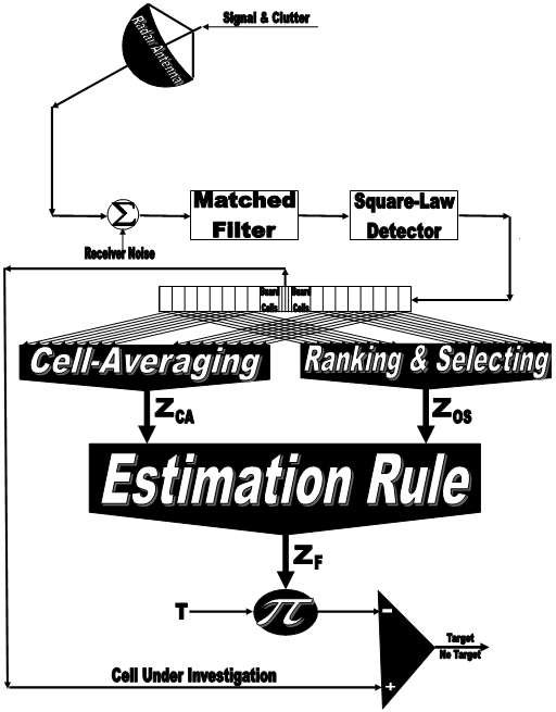 | Figure 1. The diagrammatic sketch of the modified versions of adaptive radar target detectors |
Let the input target signal and noise to the square-law detector are represented by the complex vectors u + jv and a + jb, respectively. The variables "u" and "v" represent the in-phase and quadrature components of the target signal at the square-law detector, while the corresponding components of noise are denoted by "a" and "b", respectively. The target's signal is assumed to be independent of the noise and the in-phase samples are assumed to be independent and identically distributed (IID) with the Gaussian probability density function (PDF). The output of square-law detector, normalized to the noise power, is | (1) |
The characteristic function (CF) of "ν" can be expressed as | (2) |
In the above expression, pu (u) and pa (a) denote the PDF’s of "u" and "a", respectively, "ψ" represents the noise power. From our previous assumptions, one can write the joint PDF of "a" as | (3) |
The substitution of Eq.(3) in Eq.(2) yields | (4) |
There are many PDF's for target cross section which are used to characterize fluctuating targets. The more important PDF is the so-called χ2 distribution with 2κ degrees of freedom. The χ2 model approximates a target with a large reflector and a group of small reflectors, as well as a large reflector over a small range of aspect values. The χ2 family includes the Rayleigh (Swerling cases I & II) model, the four-degree of freedom model (Swerling cases III & IV), the Weinstock model (κ <1) and the generalized model (κ a positive real number)[7]. These models are used to represent complex targets such as aircraft and have the characteristic that the distribution is more concentrated about the mean as the value of the parameter κ is increased. This distribution has a PDF given by[5] | (5) |
In the above expression,  represents the average cross section over all target fluctuations and U(.) denotes unit step function. When κ=1, the PDF of Eq.(5) reduces to the exponential or Rayleigh power distribution that applies to the Swerling case I. Swerling cases II, III, and IV correspond to κ=M, 2, and 2M, respectively. Here, we are concerned only with single sweep case (M=1). It is finally of importance to note that the χ2 distribution with 2κ degrees of freedom can be obtained by adding squared magnitude of κ complex Gaussian random variables. In other words, if κ=1, then σ may be generated as σ=w12+w22, where wi’s are IID Gaussian random variables, each with zero mean and ‾σ/2 variance. The magnitude of the in-phase component u (u=w1) has a PDF given by
 | (6) |
The substitution of Eq.(6) into Eq.(4) yields | (7) |
If we let the average signal-to-noise ratio (SNR) α/ψ=S and after performing the specified integration, Eq.(7) takes the form: | (8) |
For the sake of simplicity, the above equation can be put in another clarified form as | (9) |
The PDF of the output of the ith test tap is given by the Laplace inverse of Eq.(9), after making some minor modifications. If the ith test tap contains noise alone, we let S=0, that is the average noise power at the receiver input is "ψ". If the ith range cell contains a return from the primary target, Eq,(9) rests as it is where S represents the strength of the target return at the receiver input. On the other hand, if the ith test cell is corrupted by interfering target return, S must be changed to I, where I denotes the interference-to-noise (INR) at the receiver input. Finally, if the ith cell is immersed in clutter, S is altered to C where C denotes clutter-to-noise ratio (CNR). Implementing the generalized likelihood ratio test, the system decides the absence or the presence of a radar target according to whether | (10) |
where ν denotes the content of the cell under test, Zf represents the final noise level estimate, and T is a constant scale factor used to achieve the required rate of false alarm. Our approach in analysing a CFAR processor is to evaluate its probability of detection which is defined as | (11) |
In terms of the PDF of ν and Zf, Eq.(11) can be formulated as | (12) |
Fzf represents the cumulative distribution function (CDF) of Zf. By taking the Laplace inverse of Eq.(9) and substituting it in the previous formula, one obtains | (13) |
ΨZ (.) denotes the Laplace transformation of the CDF of the random variable Zf. The result of this analysis reveals that the Laplace transformation of the CDF of the final noise level estimate is the backbone of the CFAR performance evaluation. In terms of the CF of Zf, ΨZ (.) can be calculated as | (14) |
Therefore, it is required now to derive the CF of the final noise level estimate for each one of the modified versions in order to analytically evaluate its performance either in the absence or in the presence of outliers. Finally, as S tends to zero (S → 0), Eq,(13) leads to false alarm probability (Pd → Pfa)
3. Performance of CFAR Detectors in ideal Situations
The statistical model with uniform clutter background describes the classical signal situation with stationary noise in the reference window. In this model, two signal cases are of interest: (a) one target in the test cell in front of an otherwise uniform background, (b) uniform noise situation throughout the reference window. In both cases, the noise in neighbourhood samples has a uniform statistic, i.e., the random variables Y1, Y2, …...., YN in the reference window are assumed to be statistically independent and identically distributed. In the absence of the target case, the random variable ν of the tested cell is assumed to be statistically independent of the neighbourhood and subject to the same distribution as the random variables Yi’s.The essence of CFAR is to compare the decision statistic ν with an adaptive threshold TZf. The threshold coefficient T is a constant scale factor used to achieve the desired false alarm rate for a given window size N when the background noise is homogeneous. The statistic Zf is a random variable whose distribution depends upon the particular CFAR scheme and the underlying distribution of each of the reference range samples. As shown in the previous section, the characteristic function of the noise power level estimate ‘Zf’ is the fundamental parameter that determines the processor performance either in homogeneous or non-homogeneous background environments. Therefore, our scope in the following subsections is to calculate this important parameter for the CFAR algorithms under consideration.
3.1. Cell-Averaging (CA) Detector
A simple approach to achieve the CFAR condition is to set the detection threshold on the basis of the average noise power in a given number of reference cells where each of these cells is assumed to contain no targets. Such a scheme is denoted as cell-averaging (CA) CFAR processor. This detector is specifically tailored to provide good estimates of the noise power in the exponential PDF. Such estimation of the noise power is a sufficient statistic for the unknown noise power ψ under the assumption of exponentially distributed homogeneous background. In other words, the noise power is estimated as  | (15) |
Under the assumption that the surrounding range cells contain independent Gaussian noise samples with the same variance, ZCA is the maximum likelihood estimate of the common variance. In the absence of the radar target, each cell of the reference window has a CF of the same form as that of ν with the exception that A must be set to zero. Therefore, eliminating A in Eq.(9) leads to | (16) |
The rationale for the CA type of CFAR schemes is that by choosing the mean, the optimum CFAR processor in a homogeneous background when the reference cells contain IID observations governed by exponential distribution is achieved. As the size of the reference window increases, its detection performance approaches that of the optimum processor which is an algorithm based in its operation on a fixed threshold.It is obviously of value to have some idea about the loss of detection power for a proposed CFAR scheme relative to the optimum processor for a homogeneous noise background. The simplest and more efficient method is that based on the average detection threshold (ADT) since the threshold and detection probability are closely related to each other. It is well known that as the threshold increases, the detection probability decreases accordingly and vice versa. Therefore, we use the concept of ADT to compare different CFAR processing techniques. Mathematically, this ADT is defined as[9] | (17) |
The substitution of Eq.(16) into Eq.(17) gives | (18) |
3.2. Ordered-Statistic (OS) Detector
The performance of CA-CFAR detector degrades rapidly in non-ideal conditions caused by multiple targets and nonuniform clutter. The ordered-statistic (OS) CFAR is an alternative to the CA processor. It trades a small loss in detection performance, relative to the CA scheme, in ideal situations for much less performance degradation in nonhomogeneous background environments.Order statistics characterize amplitude information by ranking observations in which differently ranked outputs can estimate different statistical properties of the distribution from which they stem. The order statistic corresponding to a rank K is found by taking the set of N observations Y1, Y2, ……., YN and ordering them with respect to increasing magnitude in such a way that  | (19) |
Y(K) represents the Kth order statistic. The central idea of OS-CFAR procedure is to select one certain value from the above sequence and to use it as an estimate ZOS for the average clutter power as observed in the reference window. Thus, | (20) |
We will denote by OS(K) the OS scheme with parameter K. The value of K is generally chosen in such a way that the detection of radar target in homogeneous background environment is maximized.In order to analyse the processor detection performance in uniform clutter background, the CF of the random variable ZOS is required. To evaluate this quantity, we start with the homogeneous representation of the CDF of the noise estimate which has a formula given by[12] | (21) |
with  | (22) |
By substituting Eq.(22) into Eq.(21) and taking the Laplace transformation, one obtains | (23) |
By using Eq.(14) and Eq.(23) in the definition of ADT, we have | (24) |
The processor detection performance is easily evaluated once the CF of the noise level estimate ZOS is obtained. Finally, a desirable CFAR scheme would of course be one that is insensitive to changes in the total noise power within the cells of the reference window so that a constant false alarm rate is maintained. This is actually the case of all architectures under consideration.
3.3. Modified Versions
Excessive numbers of false alarms in the CA processor at clutter edges and degradation of its detection performance in multiple target environments are the prime motivations for exploring other CFAR schemes. Since CA technique is the optimum CFAR processor given that the background is homogeneous and the reference cells contain independent and identically distributed observations governed by an exponential distribution, it is intuitive to use this identity in developing new versions. Additionally, the OS scheme has its immunity to the presence of interfering target returns amongst the contents of the reference window used for noise level estimation. For this important property of OS, it is of interest to include its basics in the development of the new CFAR schemes. Here, we are interesting in analysing three of such modified versions; namely; Mean-Level (ML), Maximum (MX) and Minimum (MN) operators.
3.3.1. Mean-Level (ML)-CFAR
The contents of the N reference samples feed two signal processors simultaneously. The first one of them estimates the unknown noise power employing the CA technique while the other does the same thing using OS basis. The two estimates are combined through the meal-level operation to estimate the final noise power level. Thus,  | (25) |
Where ZCA and ZOS are as previously given in Eqs.(15, 20), respectively. The ω-domain representation of Zf, which is ZML in this case, is characterized by a CF of the form | (26) |
All the parameters of the above equation are previously evaluated as shown in Eqs,(14, 16, 23) . Therefore, the processor detection performance is completely determined as Eq.(13) demonstrates. Finally, the ADT of this version of CFAR schemes can be easily computed and the result takes the form | (27) |
3.3.2. Maximum (MX)-CFAR
This version was specifically aimed at reducing the number of excessive false alarms at clutter edges. The final noise power is estimated from the larger of the two separate noise level estimates computed for the CA and OS schemes. For this procedure of CFAR, we have  | (28) |
In this case, Zf has a CDF given by[10] | (29) |
In order to analyse this version, the Laplace transformation of the above formula must be computed. To carry out this task, we start with Eq.(21) and use it in Eq.(28) which becomes | (30) |
By taking the Laplace transformation of Eq.(30), one obtains | (31) |
The substitution of Eq,(31) into the definition of Pd yields to the evaluation of the performance of the CFAR under investigation. On the other hand, the ADT of the underlined scheme is | (32) |
3.3.3. Minimum (MN)-CFAR
In order to prevent the suppression of closely spaced targets, the minimum version has been introduced. While testing for target presence at a particular range, the processor must not be influenced by the outlying target echoes. In MN-CFAR scheme, the noise power estimate is achieved by taking the smaller of ZCA and ZOS as depicted in[5]. That is, | (33) |
In this case, the final noise level estimate has a CDF given by[12] | (34) |
It is obvious from the above formula that there is a direct relation between the detection performance of MX-CFAR and that of MN-CFAR. This means that once the performance of MX operation is calculated, the performance of MN version is easily obtained. In ω-domain, Eq.(34) takes the form | (35) |
Consequently, the ADT has a similar formula as that given by Eq.(35). Thus, it is formulated as | (36) |
3.4. Processor Performance Assessment
In this section, we give some representative numerical results, which will give an indication of the tightness of our previous analytical expressions. Since the performance of OS-CFAR is strongly dependent on the ranking parameter K, we choose the value that corresponds to the optimum detection performance in uniform noise background which is 21 for N=24[9].  | Figure 2. Thresholding constant as a function of the ordering parameter of CFAR algorithms when N=24 |
 | Figure 3. Average detection threshold (ADT)of CFAR processors as a function of ranking parameter K when N=24 |
 | Figure 4. Receiver operating characteristic (ROC) of CFAR processors in an ideal environment when N=24 |
 | Figure 5. Single pulse detection performance of CFAR schemes in homogeneous situation for N=24 |
 | Figure 6. Single pulse detection performance of CFAR schemes with fixed value for the ranking order parameter “K” and operating in homogeneous environment when N-24 |
 | Figure 7. Single pulse detection performance of CFAR schemes with fixed “K” and operating in an ideal environment when N=24 and K=10 |
The actual probability of detection achieved by the modified versions of CFAR detectors in an ideal environment has been evaluated by means of computer simulation, where their derived analytical formulas are transferred into a sequence of programs using C++ scientific language. The detection performances of the underlined detectors are also compared with that of CA- and OS-CFAR detectors to see to what extent the performance of the new versions improves. Since the constant scale factor T represents the fundamental quantity in the evaluation of the processor performance, we start our presentation by running the program that concerns with the determination of T given that the false alarm probability is held fixed and the operating environment is free of interferers. The results of this program are depicted in Fig.(2) which illustrates the thresholding constant T as a function of the ranking order parameter K for CA, OS, and their modified versions. Two values for Pfa (10-8 & 10-4) are simulated. Since CA estimates its noise power by averaging the candidates of the reference set, the constant scale factor that this estimation must be multiplied, to achieve a prescribed rate of false alarm, becomes independent of K. This is actually the case of our presentation. It is of importance to note that as Pfa decreases, the detection threshold increases, given that the size of the reference set is held unchanged. The displayed results demonstrate this property for all the CFAR processors considered here. The behaviour of T for OS technique is as previously shown in the literature[9]. Since the MX version selects the maximum of the CA and OS noise level estimates, its noise power estimate equals that of OS for K=N, and consequently its scaling factor T coincides with that of OS at this value of K. As K goes in the reverse direction (Kfa is plotted in Fig.(3) for the processing schemes under investigation. It is obvious that ADT=T for the CA technique and hence it rests unchanged as K varies. On the other hand, the behaviour of ADT for the OS technique is as well known in the literature[12]. Since there is a direct proportionality between the ADT and T, the average detection threshold behaves as T with minor changes and this is common for all the CFAR presented in this paper.Let us turn our attention to the receiver operating characteristics (ROC's) of the processors under consideration. This behaviour describes the variation of the detection probability as a function of the false alarm probability given that the SNR is held constant. Fig,(4) displays the results of these characteristics for the considered schemes for two values for the primary target SNR (5 & 10dB). The displayed results show that the processor detection performance improves, in a logarithmic linear fashion, as the rate of false alarm decreases and this is common for all the CFAR processors. It is well-known that the CA scheme is the optimum processor that has the highest detection performance in homogeneous situation. However, the performance of the modified versions outweighs that of the CA detector for some values for the ranking order parameter K as noted from the results of the figure under examination. The degree of superiority varies from one modified version to another. The ML operation has the top and the MN procedure has the lowest and this classification is verified for the two chosen values of SNR. To confirm this property, the detection probability as a function of SNR is drawn in Fig.(5) for CA, OS, and their modified versions for two fixed values of false alarm rate. It can be seen that the ML-CFAR achieves the highest detection performance and the MN-CFAR has the lowest degree of improvement. All the modified techniques give detection performance better than that of CA- and OS-CFAR schemes. Finally, we conclude that, the performance of the ML-CFAR is the best one among the five detectors, with MX-CFAR comes next to it, then MN-CFAR, after that CA-CFAR, and OS-CFAR gives the worst homogeneous detection performance in the selected group. This classification is obtained taking into account that each detector selects its ranking order parameter K that achieves its highest detection performance. Now, let us show the influence of the ranking order parameter K on the homogeneous performance of the detectors under consideration. Figs.(6-7) demonstrate the effect of fixing K for all the schemes. In the first plot, K is taken as that corresponding to the maximum performance of OS (K=21), while in the other figure, K is randomly chosen (K=10). The variation of the curves of Fig.(6) indicates that the ML version is still the king of the group and the processor OS has the worst detection performance. The behaviour of MN developing detector acts as the conventional CA scheme while the MX procedure gives lower performance than CA but still higher than that of OS processor. On the other hand, the results of Fig.(7) behave as those of the previous figure except that the gap between the family of CA and the family of OS becomes larger. The candidates of CA family include ML and MX modified versions, while the family of OS incorporates MN only. Additionally, it is obvious that as the false alarm decreases, the width of the gap between these families increases. Moreover, the MX developed processor gives higher detection performance than CA for this value of the ranking order parameter K (K=10).
4. Performance of CFAR Schemes in Non-homogeneous Environments
The CFAR algorithms were originally developed using a statistical model of uniform background noise. However, this is not representative of real situations. It is impossible to describe all radar working conditions by a single model, yet consideration of a larger number of different situations might be confusing. For these reasons, three different signal situations are selected: uniform clutter, clutter edges and multiple targets. The performance of the CFAR algorithms for uniform clutter model was completely evaluated in the previous section. Clutter edges, on the other hand, are used to describe transition areas between regions with very different noise characteristics[8]. This situation occurs when the total noise power received within a single reference window changes abruptly. The presence of such a clutter edge may result in severe performance degradation in an adaptive threshold scheme leading to excessive false alarms or serious target masking depending upon whether the cell under test is a sample from clutter background or from relatively clear background with target return, respectively. On the other hand, multiple target situations occur occasionally in radar signal processing when two or more targets are at a very similar range. The consequent masking of one target by the others is called suppression. These interferers can arise from either real object returns or pulsed noise jamming. From a statistical point of view, this implies that the reference samples, although still independent of one another, are no longer identically distributed.
4.1. Cell-Averaging (CA) Detector
In order to analyse the CFAR detection performance when the candidates of the reference window no longer contain radar returns from a homogeneous background, as in the case of clutter edges, the assumption of statistical independence of the reference cells is retained. Let us assume that the reference set contains R cells from clutter background with noise power ψ(1+C), with C denotes the clutter-to-thermal noise ratio (CNR), and N-R cells from clear background with noise power "ψ". Thus, the estimated total noise power level is obtained from | (37) |
The random variable ZC representing the clutter return and that denoting the clear background Zc have CF's given by a similar form as that indicated in Eq.(16) after minor changing of its parameters. Since the candidates of each type are assumed to be statistically independent, we have  | (38) |
Since ZC and Zc are statistically independent, the CF of ZCA is simply the product of the individual CF's of ZC and Zc. Therefore, assuming that the cell under investigation is from clear background, the false alarm probability has a formula given by | (39) |
As the window sweeps over the range cells, more cells from clutter background enter into the reference window. When the cell under test comes from clutter background, the probability of false alarm takes the form; | (40) |
Another situation of non-homogeneity is the case of multiple targets. In our analysis and study of this situation for which the reference cells don’t follow a single common PDF, we are concerned with increases in the value of ψ for some isolated reference cells due to the presence of secondary targets. The amplitudes of all the targets present amongst the candidates of the reference window are assumed to be of the same strength and to fluctuate in accordance with SWII fluctuation model as the primary target. The interference-to-noise ratio (INR) for each of the spurious targets is taken as a common parameter and is denoted by I. Thus, for reference cells containing extraneous target returns, the total background noise power is ψ(1+I), while the remaining reference cells have identical noise power of ψ value. The determination of the detection probability is similar to the one presented above for the clutter power transitions with some changes in the definition of the parameters. R will now represent the number of outlying target returns amongst the contents of the reference set.
4.2. Ordered-Statistic (OS) Detector
In order to analyse the processor performance in non-homogeneous background, we follow the same steps as those presented for CA technique. Consider the same previously stated situation where there are R reference samples contaminated by clutter returns, each with power level ψ(1+C), and the remaining N-R reference cells contain thermal noise only with power level ψ. Under these assumptions, the Kth ordered sample, which represents the noise power level estimate in the OS detector, has a CDF given by[13] | (41) |
Fc(.) denotes the CDF of the reference cell that contains a clear background and FC(.) denotes the same thing for the reference cell that belongs to clutter. Mathematically, these functions can be formulated as: | (42) |
By substituting Eq.(42) into Eq.(41) and taking the Laplace transformation of its resulting formula, one obtains | (43) |
Once the ω-domain representation of the CDF of the noise power level estimate is calculated, the processor performance evaluation becomes an easy task, as we have previously shown, where the false alarm and detection probabilities are completely dependent on this transformation. In the presence of interferers, the OS-CFAR processor performance is highly dependent upon the value of K. For example, if a single extraneous target appears in the reference window of appreciable magnitude, it occupies the highest ranked cell with high probability. If K is chosen to be N, the estimate will almost always set the threshold based on the value of interfering target. This increases the overall threshold and may lead to a target miss. If, on the other hand, K is chosen to be less than the maximum value, the OS-CFAR scheme will be influenced only slightly for up to N-K spurious targets.
4.3. Modified Versions
4.3.1. Mean-Level (ML)-CFAR
In this type of modified versions, the noise level estimate employing CA technique and that using OS procedure are combined through the mean-level operation to obtain the final noise power level estimate. The purpose of this processing is to improve the processor performance in the absence as well as in the presence of outlying targets. In the case where the operating environment has a clutter edge, the evaluation of the processor false alarm rate follows the same procedure as in CA and OS cases. Using Eqs.( 39,14,43) in Eq.(26), the Laplace transformation of the CDF of the noise level estimate of this processor can be computed and consequently, the evaluation of false alarm rate in clutter edges and the detection performance in multiple-target situations are completely determined.
4.3.2. Maximum (MX)-CFAR
As previously stated, for MX-CFAR, the content of the cell under test must be greater than both the CA-CFAR threshold and the OS-CFAR threshold to declare the presence of a target, which is equivalent to choosing the maximum value of the CA-CFAR and the OS-CFAR thresholds and compare it with the target cell (cell under investigation). For the processor performance to be evaluated, let us go to calculate the Laplace transformation of the CDF of the final noise power level estimate of the underlined detector. By substituting Eq.(41) in Eq.(29) and transferring it to the ω-domain representation, we have | (44) |
Again, once the Laplace transformation of the CDF of the noise level estimate is achieved, the false alarm rate performance in the presence of clutter edges and the detection probability in the presence of spurious targets are completely known since ΨMX(ω) represents the backbone of their evaluation.
4.3.3. Minimum (MN)-CFAR
As the case of MN-CFAR, the content of the target cell should be greater than the CA-CFAR threshold or the OS-CFAR threshold to declare a target present, which is equivalent to choosing the minimum value of the CA-CFAR and the OS-CFAR thresholds and compare it with the primary target return to indicate its presence. As Eq.(35) demonstrates, there is a direct relation between the performance evaluation of this processor and that of the MX-CFAR scheme. This means that once the false alarm rate probability in clutter edges situation and the detection probability in multiple target environments are calculated for the MX-CFAR version, their evaluations in the case of MN-CFAR detector are automatically known given that the performances of the original processors (CA and OS) are completely determined. This is actually the case of our treatment.  | Figure 8. False alarm rate performance of CFAR schemes in the presence of clutter edges with ONR=10dB for N=24, and design Pfa=1.0E-6 |
 | Figure 9. False alarm rate performance of CFAR schemes operating in clutter edge environment with CNR=15dB for N=24,K=21,and design Pfa=1.0E-6 |
4.4. Processor Performance Assessment
Here, we provide a variety of numerical results for the performance of CA- and OS-CFAR processors as well as their modified versions in the case where the operating environment contains either clutter edge or a number of outlying targets. Since the optimum value of K, for a reference window of size 24, is 21, we have assumed that there are three interfering target returns amongst the contents of the estimation cells. This value of extraneous target returns is the maximum allowable value before the OS performance degradation occurs. Our results are obtained for a possible practical situation where the primary and the secondary interfering targets fluctuate in accordance SWII model and of equal target return strength (INR=SNR). The design probability of false alarm is maintained at its previous value (Pfa=10-6). The false alarm performance of the underlined CFAR processors when the reference window contains a clutter edge is numerically evaluated. Fig.(8) illustrates the actual value of false alarm rate in the presence of clutter edge when there are R cells immersed in clutter. The result in this figure is obtained for a clutter to noise ratio (CNR) of 10 dB and for the design value of the ranking order parameter K for each scheme. The displayed results show that the OS(21) has the lowest false alarm rate at clutter edge and is followed by CA, MN(18), MX(15), and ML(17) comes the last one in the concerned group. In other words, OS(21) has the best performance among all the underlined CFAR processors in the presence of non-uniform clutter. To show the effect of changing K on the processor performance, Fig.(9) illustrates the same thing as the previous figure except that K is held fixed (K=21) for all the schemes and the CNR is changed to 15dB. In this situation, the MX version gives the best false alarm rate and the OS comes next. The CA and MN have the worst rate of false alarm under these circumstances. Therefore, the selection of the ranking order parameter K plays an important rule in the reaction of the processor to the environmental conditions.  | Figure 10. Single pulse multiple target detection performance of CFAR schemes for CFAR schemes for N=24,and R=3 |
 | Figure 11. Single pulse detection performance of CFAR processors for N=24, K=21, R=3, and Pfa=1.1E-6 |
 | Figure 12. Multiple target detection performance of CFAR processors with fixed value for the ranking order parameter “K” when N=24, M=1, K=18, and R=5 |
 | Figure 13. Actual false alarm rate performance of CFAR schemes in target multiplicity environment for N=24, and R=3 |
 | Figure 14. Required SNR to achieve an operating point (1.0E-6, Pd) of CFAR schemes operating in multiple target environment with R=3,and N=24 |
The presence of multiple targets is another case in studying the non-homogeneous performance of the modified versions. Since the maximum allowable value for the interfering target returns that may exist amongst the candidates of the reference window is 3 (R ≤ N-K), the results in Fig.(10) depict the detection performance of the CFAR schemes under consideration for this situation of operating conditions. The displayed curves are obtained for a possible practical application of equal strengths for the outlying as well as the primary target. Two values for the design false alarm rate are taken into account to show the influence of this rate on the behaviour of the CFAR scheme in detecting the radar target. From the variations of the underlined curves, it is obvious that the CA algorithm has the worst multiple target detection performance and all the developed versions give much better performance than it. However, the ML and MX versions have lower values for the detection probability than the OS procedure. Additionally, the MN detector is the only one that has a multiple-target detection performance higher than that of the OS scheme. Moreover, the shown results reckoned the well-known identity of the CFAR signal processing that the processor detection performance improves as its design false alarm rate increases. In order to compare the reaction of the CFAR processor to the ideal environment against its behaviour in non-homogeneous situation, Fig.(11) illustrates the detection performance of the under investigated processors in the absence as well as in the presence of interferers for a fixed value of K. As a reference for this comparison, the performance of the optimum detector is also included in that figure. The OS(21) has the worst homogeneous performance and the ML version has the highest one, while MN gives the same performance as the CA technique. The MX version has a performance that is higher than the OS scheme but less than the CA processor. On the other hand, the OS gives the highest detection performance when operating in an environment contaminated with three interfering target returns. As expected, the CA has the worst performance. For the modified detectors, the MN version has a multiple target performance which is close to that of OS, the MX gives the worst, relative to its candidates, and the ML lies in between. These concluded remarks are associated with the steady-state behaviour of the underlined processors. Fig.(12) deals with the detection performance of CA and OS techniques along with their extended versions in the presence of spurious targets when there are five contaminated samples. Two design values for the false alarm rate are assumed and the ranking order parameter is held constant at 18 (K=18). The examination of the curves of this figure leads to the same concluded observations as the previous results with minor degradation. It is of interesting to see to what extent the presence of interferers affect the rate of false alarm of the adaptive scheme of detection. Fig.(13) displays the actual false alarm probability of the underlined processor as a function of the strength of interference when the design rate of false alarm takes the values of 10-8 and 10-4. The results of this figure show that the false alarm rate performance of the CA, MX, and ML processors degrades as the strength of the interfering target return (INR) increases. On the other hand, the OS and MN schemes are the only ones that are capable of maintaining the rate of false alarm constant, especially, when the INR becomes stronger. This result is expected since the largest interfering target returns occupy the top ranked cells and therefore they are not incorporated in the estimation of the background noise power level. In other words, the noise estimate is free of extraneous target returns and therefore it represents the homogeneous background environment. Finally, the value of the SNR, that is required to satisfy a pre-assigned value for the detection probability when the rate of false alarm is held constant, is plotted in Fig.(14). The operating environment is assumed to be free of any interferer as well as in the case where the environment is contaminated with three interferers of the same strength as the target under test. In homogeneous situation, the ML(17) requires the minimum SNR to achieve an indicated value for the detection probability. MX(15) comes in the second class and followed by MN(18). CA processor comes next and the conventional OS technique requires the highest SNR to achieve the same operating point. On the other hand, the MN(18) achieves the specified value of detection probability with the minimum SNR when the operating environment is of multiple-targets. In this situation, the OS scheme behaves like MN(18) but with higher values of SNR. The ML(17) achieves only some values for Pd and unable to achieve the others since its multiple target detection performance is asymptotically constant at some value which is less than the required ones. The same remark can be said about the behaviour of MX(15) and CA procedures.
5. Conclusions
In this paper, the detection probability of a radar system that utilizes new versions of adaptive detectors in deciding the presence or absence of fluctuating target in either ideal or non-ideal operating environments was analysed. Three versions of such techniques are processed and closed form expressions are derived for their detection performance. These processors include ML, MX, and MN operations on two separately noise power estimates from a reference set of N cells: one of them employs CA technique and the other uses OS basis. The analytical results have been used to develop a complete set of performance curves including thresholding constant, ROC’s, false alarm rate in clutter edges, detection probability in homogeneous and multiple target situations, required SNR to achieve a prescribed values of Pfa and Pd, and the variation of false alarm rate with the strength of interfering targets that may exist amongst the contents of the estimation set. As expected, the detection performance of the modified versions outweighs that of CA scheme, either in homogeneous or in multiple target environments, for some selected values for the ranking order parameter. From the interference point of view, the considered detectors are partitioned into two families: the CA family and the OS one. The family of CA incorporates ML and MX while that of OS includes MN only. The performance of OS family outweighs that of CA family in non-homogeneous situations. In addition, this family is capable of maintaining a constant rate of false alarm, irrespective to the interference level, in the case where the spurious target returns occupy the top ranked cells and they are within their allowable values. As a final conclusion, the detection performance of the modified versions is related to the ranking order parameter, the target model, the average power of the target, and the environmental operating conditions.
References
| [1] | Rickard, J. T. & Dillard, G. M. (1977), “Adaptive detection algorithm for multiple target situations”, IEEE Transactions on Aerospace and Electronic Systems, AES-13, (July 1977), pp. 338-343. |
| [2] | Mclane, P. J., Wittke, P. H. & K-S IP. C. (1982), “Threshold control for automatic detection in radar systems”, IEEE Transactions on Aerospace and Electronic Systems, AES-18, (Mar. 1982), pp. 242-248. |
| [3] | P. P. Gandhi and S. A. Kassam (1988), "Analysis of CFAR Processors in nonhomogeneous background", IEEE Transactions on Aerospace and Electronic Systems, AES-24, pp. 427-445, 1988. |
| [4] | El Mashade, M. B. (1994), “M-sweeps detection analysis of cell-averaging CFAR processors in multiple target situations”, IEE Proc.-Radar, Sonar Navig., Vol.141, No.2, (April 1994), pp. 103-108. |
| [5] | El Mashade, M. B. (2000), “Detection analysis of CA family of adaptive radar schemes processing M-correlated sweeps in homogeneous and multiple target environments”, Signal Processing ,“ELSEVIER”, Vol. 80, (2000), pp. 787-801 |
| [6] | Lei Zhao, Weixian Liu, Jeffery S. Fu, Sin Yong Seow and Xin Wu (2001), ‘Two New CFAR Detectors Based on Or-Algorithm and And-Algorithm’; Proceedings of SCOReD 2001, KL, Malaysia, 2001, pp. 31-34. |
| [7] | El Mashade, M. B. (2002), “Target Multiplicity Performance analysis of radar CFAR detection techniques for partially correlated chi-square targets”, Int. J. Electron. Commun. (AEŰ), Vol.56, No.2, (April 2002), pp. 84-98. |
| [8] | Biao Chen, Pramod K. Varshney & James H. Michels (2003), "Adaptive CFAR Detection for Clutter-Edge Heterogeneity Using Bayesian Inference", IEEE Transactions on Aerospace and Electronic Systems Vol. 39, No. 4, October 2003, pp.1462-1470. |
| [9] | El Mashade, M. B. (2005), “M-Sweeps exact performance analysis of OS modified versions in nonhomogeneous environments”, IEICE Trans. Commun., Vol.E88-B, No.7, (July 2005), pp. 2918-2927 |
| [10] | El Mashade, M. B. (2006), “Analysis of cell-averaging based detectors for χ2 fluctuating targets in multitarget environments”, Journal of Electronics (China) 23 (6) (November 2006), pp. 853–863. |
| [11] | Simon Haykin (2007), “Adaptive Radar Signal Processing”, A John Wiley & Sons, Inc., Publication |
| [12] | El Mashade, M. B. (2008), “Performance analysis of OS structure of CFAR detectors in fluctuating targets environments”, Progress in Electromagnetics Research (PIER) C2 (2008) 127–158. |
| [13] | El Mashade, M. B. (2011), “Analysis of adaptive detection of moderately fluctuating radar targets in target multiplicity environments”, Journal of the Franklin Institute 348 (2011) 941–972 |
 Abstract
 Reference
 Full-Text PDF
 Full-Text HTML