1. Introduction

Beamforming using an antenna array is a promising and necessary task in the next generation wireless and mobile systems. Sensor arrays are extensively used in signal processing and their capability has made numerous applications in different fields such as radar, sonar, radio astronomy, medical diagnosis, acoustics and mobile or wireless communications. Combination of the signals collected from array sensors provides temporal and spatial analysis of wave-fields and yields directional sensitivity for the system. The important tasks considered in array signal processing are beamforming, Angle Of Arrival (AOA) or Direction Of Arrival (DOA) estimation and source tracking. Variant techniques and algorithms are available with different characteristics in efficiency, accuracy and computational costs and also numerous studies are attempting to improve these techniques or proposing new efficient methods[1, 2]. In addition to different algorithms, structure of array plays a key role in array signal processing. Various arrangements are studied and have demonstrated significant effects on the performance of the system.

Uniform Linear Array (ULA) is the most common configuration used for array processing investigations. This geometry is simple in analysis and implementation and provides a good accuracy via formation of narrow beams during beamforming. However, ULA can analyse the surrounding wave-fields in a particular dimension and provides one-Dimensional (1-D) coverage. Furthermore, ULA cannot give a uniform performance in all directions. DOA estimation and beamforming with ULA leads to weak results at the angles close to the array endfires. Therefore, other array geometries are investigated to obtain a uniform performance. Uniform Circular Array (UCA) is another common geometry used for array processing. This structure has further complexity in implementation as well as analysis with respect to ULA. Instead, UCA can provide 2-D coverage and present uniform performance in all directions. Beams in UCA are wider than ULA and this affects resolution of the array[3, 4]. Concentric Circular Array (CCA) or multi-ring arrays are other configurations that provide more flexibility in size and width of the obtained beams[5]. However, the required computational complexity for analysing the array structure increases in CCAs. Planar arrays are also used for 2-D and more precise beam-pattern generation. 3-D arrays and conformal arrays may be used in particular applications to provide M-D performance and conformity with the vehicle or system they are integrated with it[3]. However, these structures are complicated in calculations as well as implementation and research works are attending to find and develop simple arrangements which present better efficiency and perform uniform in all directions. Combination of linear arrays is considered in literature and has shown improvements in array performance specially the accuracy of DOA estimation algorithms. Some of these structures are parallel linear arrays and Displaced Sensor Arrays (DSAs), L-shaped and two L-shaped arrays, V-shaped, Y-shaped, Uniform Rectangular Arrays (URA), hexagonal arrays and so on[6-11]. Each configuration has particular properties and capabilities. These geometries are often used for DOA estimation and they can provide at least 2-D DOA estimation capability. In Ref.[11] different types of array structures (ULA, UCA and URA) for smart antennas, DOA estimation and beamforming have been examined.

This paper is following the authors’ earlier papers[12-14], in which a simple ULA-based geometry was introduced that could provide a significant improvement in DOA estimation capability and resolution threshold in border angles of the array endfire. In this article, by focusing on antenna beamforming, the capability of Shirvani-Akbari Array (SAA) which adds two elements to the ULA in top and bottom of the array axis is investigated. Two well-known adaptive beamforming techniques, Least Mean Squares (LMS) and Normalized Least Mean Squares (NLMS) are exploited for evaluation of SAA performance. Simulation results are compared with the results of beamforming using conventional ULA. Numerical results show higher accuracy and also uniform performance through this new proposed array with respect to conventional ULA.

The rest of paper is organized as follows. Section 2 describes signal model for array processing through ULA as well as SAA. A brief overview of adaptive beamforming techniques and description of LMS and NLMS algorithms are stated in sections 3, 4, respectively. In section 5, simulation results using MATLAB software are presented and the performance of both arrays is compared together. Finally, conclusion remarks are given in section 6.

2. Signal Model for Array Processing

Fig. 1 depicts the block diagram of an adaptive array system. System is composed of an array of sensors, complex weights, summer and a signal processing unit.

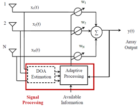Figure 1. Block diagram of an adaptive array system

In this article, antenna elements are configured as ULA and SAA, demonstrated in Fig. 2, 3, respectively.

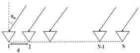Figure 2. ULA geometry

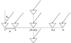Figure 3. SAA geometry

The adaptation takes place in the signal processing unit to fulfil the beamforming and adjust the complex weights in order to obtain optimized performance for the system. The weighted received signals are combined together to form the array output. In some of the beamforming techniques an iterative procedure may be required to adjust the weights. For statement of the signal model, ULA with N and SAA with N+2 antenna elements are assumed that receive M uncorrelated narrowband signals.

Received signals, can be expressed as a linear combination of incident signals and zero mean Gaussian noise with variance. The incident signals are assumed to be direct Line Of Sight (LOS) and uncorrelated with the noise. The input signal vector denoted by can be written as (1).

(1)

is vector concerning to the m-th source located at direction from the array boresight. is the steering vector or response vector of the array for direction of. For ULA, the steering vector is as:

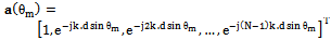(2)

where d is the inter-element spacing and.

For SAA, the steering vector has element as (3). The first N rows of for SAA are equivalent with steering vector of ULA. By addition of two remained rows with respect to ULA, is expressed as:

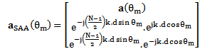(3)

For ULA, A is a matrix of steering vectors, written as:

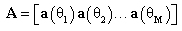(4)

For SAA, with dimensions is defined as:

(5)

The array output signal is given by:

(6)

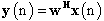
where w is the, weight vector for ULA and SAA. H denotes the Hermitian, conjugate transpose, operator and x is the received signal vector defined in (1).

3. Adaptive Array Beamforming

Beamforming that is also referred as spatial filtering is the process of adjusting the antenna radiation pattern so that the antenna focuses energy towards Signal Of Interest (SOI) and nulls directed to Signals Not Of Interest (SNOIs). This task can be fulfilled through different approaches. Although some earlier techniques such as classical beamforming or fixed-beam methods carry out this process with lower complexity, adaptive beamforming techniques are more capable. These methods adjust array weights dynamically with respect to signal environment and perform interference mitigation as well as desired signal tracking. Therefore, adaptive beamforming methods have been more considerable in recent years.

In an overview, adaptive algorithms are classified in two categories: non-blind and blind algorithms. Adaptive beamforming techniques generally need some initial information about the signal characteristics to obtain an appropriate performance. This initial information is provided via a reference signal, DOA estimation methods or some particular properties of the desired signal. The beamforming methods that utilize a reference signal, known as training sequence, are called training-based or non-blind algorithms. LMS and its variants, Recursive Least Squares (RLS) and Sample Matrix Inversion (SMI) are training-based algorithms. Blind algorithms use the desired signal properties and their DOA instead of training sequences to determine the weight vector. Constant Modulus Algorithm (CMA), Decision Directed (DD), Conjugate Gradient (CG), Least Squares (LS) and Spectral self-Coherence REstoral (SCORE) are some examples of blind algorithms[2]. In this research, two popular and reliable non blind methods, LMS and NLMS are discussed and simulated in both ULA and SAA.

4. LMS and NLMS Description

LMS is an adaptation technique based on the steepest-descent method. The algorithm updates the weights recursively by estimating gradient of the error surface and changing the weights in the direction opposite to the gradient to minimize the Mean Square Error (MSE)[2,15]. Error signal is the difference between desired signal, , and array output, , computed by the expression:

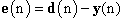(7)

According to the LMS algorithm, the final recursive equation for updating the weight vector is:

(8)

μ is the step size parameter which controls the convergence speed of the algorithm. The small step size causes slow convergence but high stability around the optimum value. On the other hand, large step size results in rapid convergence and lower stability. Hence, step size is a major parameter that makes a trade-off between the convergence speed and the LMS stability. The convergence rate of LMS also depends on the Eigen-value variance of the input correlation matrix. Variable step size algorithms are used to overcome the slow rate of convergence[16, 17]. LMS has a simple iterative equation which does not require correlation matrix calculation nor does require matrix inversions. This makes LMS a common widely-used adaptation algorithm.

According to equation (8), the correction term applied to the weight vector during LMS algorithm, is proportional to the input vector. Therefore, a gradient noise amplification problem occurs in the standard LMS algorithm. This problem can be solved by normalized LMS, in which a data dependent step size is used for adaptation. NLMS normalizes the weight vector correction term with respect to the squared Euclidean norm of the input vector at time n. So its equation can be written as:

(9)

NLMS can present better behaviour in convergence and stability than LMS[15, 18]. To prevent the convergence problem due to division by a small number, a positive constant ε may be added to the Euclidean norm of the input vector in (9) and the weight vector is computed through:

(10)

The algorithm is known as ε-NLMS and results in more reliable implementation[18]. In addition to NLMS, other versions of LMS such as sign-LMS, Constrained LMS (CLMS), Block-LMS, Partial Update LMS (PULMS) and Variable Step Size LMS (VSSLMS) have been proposed with different properties in convergence speed and efficiency. In this research, standard LMS and -NLMS algorithms are employed but new proposed SAA configuration can be applied for all above mentioned versions of LMS.

5. Numerical Results

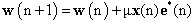
For simulation of LMS and NLMS in ULA and SAA, two arrays with 7 and 9 elements and half wavelength inter-element spacing are assumed. The performance of beamforming algorithms is evaluated in both arrays and in different signal source locations using MATLAB. Beamforming performance may be evaluated with different criteria. In this investigation, absolute value of Array Factor (AF), MSE, and Bit Error Rate (BER) are considered as performance metrics.

Fig. 4 depicts the radiation pattern when the desired signal is located at and two interference signals are assumed to be located at and the Signal to Noise Ratio (SNR) and Signal to Interference Ratio (SIR) are assumed to be 10 dB and 3 dB, respectively. Both arrays have tracked desired signal successfully and placed appropriate nulls in the interferers' directions. Beamwidth in SAA is a little wider than ULA in middle angles.

Figure 4. Array factor for the middle DOAs

Mean square error diagram during training process for both arrays is demonstrated in Fig. 5. Beamformers converge more rapidly in SAA than ULA. Fig. 6 shows the simulation results in the sense of BER for middle DOAs. According to that, exploitation of SAA in beamforming purposes leads to better results in convergence rate of beamformer and accuracy of system.

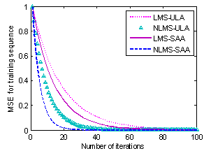Figurea 5. MSE of training sequence for the middle DOAs

To investigate beamforming performance at the angles close to the array endfire the desired signal source is assumed at and two interference signals are assumed at. Radiation pattern of both ULA and SAA arrays is shown in Fig. 7. Main lobes that are formed at border angles have better tracking accuracy at desired DOA and their widths are less than main beams formed in these directions by ULA.

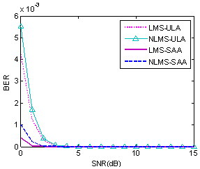
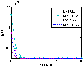Figure 6. BER versus SNR for the middle DOAs

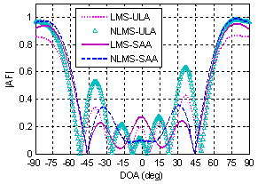Figure 7. Array factor for the border DOAs

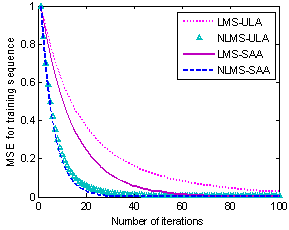Figure 8. MSE of training sequence for the border DOAs

BER diagram in this situation for both LMS and NLMS is demonstrated in Fig. 9. The level of BER is lower in SAA than ULA.

Figure 9. BER versus SNR for the border DOAs

As shown in above mentioned numerical results, the level of AF and MSE during data transmission in SAA and ULA is equivalent. Besides, exploitation of SAA in beamforming purposes leads to better results in convergence rate of beamformer and accuracy of system in the sense of BER. In addition, the performance of beamformer at boresight as well as endfire directions is better than ULA, especially in low SNRs. For higher SNRs, greater than 5dB, performance of both beamforming algorithms, LMS and NLMS, are the same for ULA as well as SAA.

6. Conclusions

In this paper, the performance of a new proposed array, SAA, for adaptive beamforming task was investigated. The new array is based on ULA configuration with two extra elements at the top and bottom of the array axis. Two popular training-based beamforming algorithms, LMS and NLMS were considered for this purpose.

Nevertheless, the performance of SAA and ULA is the same for the antenna beamforming in the case of source and interferers located at middle angles, SAA offers a well performance in detecting and resolving sources located at array endfires. Simulation results show improved convergence speed and accuracy in data transmission considering AF, MSE and BER performance metrics for the new array, especially for low SNRs. This research focused on LMS and NLMS algorithms for both ULA and SAA, but the similar procedure can be applied for other beamforming algorithms.

ACKNOWLEDGEMENTS

This work was supported by Shahid Rajaee Teacher Training University (SRTTU) under contract number 720 (20.1.1391).