-
Paper Information
- Next Paper
- Paper Submission
-
Journal Information
- About This Journal
- Editorial Board
- Current Issue
- Archive
- Author Guidelines
- Contact Us
American Journal of Signal Processing
p-ISSN: 2165-9354 e-ISSN: 2165-9362
2011; 1(1): 1-5
doi: 10.5923/j.ajsp.20110101.01
Sound Source Localization with CS Based Compressed Neural Network
 Abstract
 Reference
 Full-Text PDF
 Full-Text HTML
M. B. Dehkordi
Speech Processing Research Lab, Elec. and Comp. Eng. Dept., Yazd University, Yazd, Iran
Correspondence to: M. B. Dehkordi , Speech Processing Research Lab, Elec. and Comp. Eng. Dept., Yazd University, Yazd, Iran.
| Email: |  |
Copyright © 2012 Scientific & Academic Publishing. All Rights Reserved.
Microphone arrays are today employed to specify the sound source locations in numerous real time applications such as speech processing in large rooms or acoustic echo cancellation. Signal sources may exist in the near field or far field with respect to the microphones. Current Neural Networks (NNs) based source localization approaches assume far field narrowband sources. One of the important limitations of these NN-based approaches is making balance between computational complexity and the development of NNs; an architecture that is too large or too small will affect the performance in terms of generalization and computational cost. In the previous analysis, saliency subject has been employed to determine the most suitable structure, however, it is time-consuming and the performance is not robust. In this paper, a family of new algorithms for compression of NNs is presented based on Compressive Sampling (CS) theory. The proposed framework makes it possible to find a sparse structure for NNs, and then the designed neural network is compressed by using CS. The key difference between our algorithm and the state-of-the-art techniques is that the mapping is continuously done using the most effective features; therefore, the proposed method has a fast convergence. The empirical work demonstrates that the proposed algorithm is an effective alternative to traditional methods in terms of accuracy and computational complexity.
Keywords: Sampling, Sound Source, Neural Network, Pruning, Multilayer Perceptron, Greedy Algorithms
Cite this paper: M. B. Dehkordi , "Sound Source Localization with CS Based Compressed Neural Network", American Journal of Signal Processing, Vol. 1 No. 1, 2011, pp. 1-5. doi: 10.5923/j.ajsp.20110101.01.
Article Outline
1. Introduction
- Location of a sound source is an important piece of information in speech signal processing applications. In the sound source localization techniques, location of the source has to be estimated automatically by calculating the direction of the received signal[1]. Most algorithms for these calculations are computationally intensive and difficult for real time implementation[2]. Neural network based techniques have been proposed to overcome the computational complexity problem by exploiting their massive parallelism[3, 4]. These techniques usually assume narrowband far field source signal, which is not always applicable[2]. In this paper, we design a system that estimates the direction-of-arrival (DOA) (direction of received signal) for far field and near field wide band sources. The proposed system uses feature extraction followed by a neural network. Feature extraction is the process of selection of the useful data for estimation of DOA. The estimation is performed by the use CS. The neural network, which performs the pattern recognition step, computes the DOA to locate the sound source. The important key insight is the use of the instant neous cross-power spectrum at each pair of sensors. Instantaneous cross-power spectrum means the cross-power spectrum calculated without any averaging over realizations. This step calculates the discrete Fourier transform (DFT) of the signals at all sensors. In the compressive sampling step K coefficients of this DFT transforms are selected, and then multiplies the DFT coefficients at these selected frequencies using the complex conjugate of the coefficients in the neighboring sensors. In comparison to the other cross- power spectrum estimation techniques (which multiply each pair of DFT coefficients and average the results), we have reduced the computational complexity. After this step we have compressed the neural network that is designed with these feature vectors. We propose a family of new algorithms based on CS to achieve this. The main advantage of this framework is that these algorithms are capable of iteratively building up the sparse topology, while maintaining the training accuracy of the original larger architecture. Experimental and simulation results showed that by use of NNs and CS we can design a compressed neural network for locating the sound source with acceptable accuracy.The remainder of the paper is organized as follows. The next section presents a review of techniques for sound source localization. Section III explains feature selection and discusses the training and testing procedures of our sound source localization technique. Section IV describes traditional pruning algorithms and compressive sampling theory and section V contains the details of the new network pruning approach by describing the link between pruning NNs and CS and the introduction two definitions for different sparse matrices. Experimental results are illustrated in Section VI while VII concludes the paper.
2. Sound Source Localization
- Sound source localization is performed by the use of DOA. The assumption of far field sources remains true while the distance between source and reference microphone is larger than
 [2] fig. 1. In this equation
  is the minimum wavelength of the source signal, and D is the microphone array length. With this condition, incoming waves are approximately planar. So, the time delay of the received signal between the reference microphone and the
  microphone would be [15]:
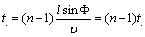 | (1) |
 is the distance between two microphones,
  is the DOA, and
  is the velocity of sound in air. Therefore,
  is the amount of time that the signal traverses the distance between any two neighboring microphones, Figure. 1 and 2 illustrates this fact.
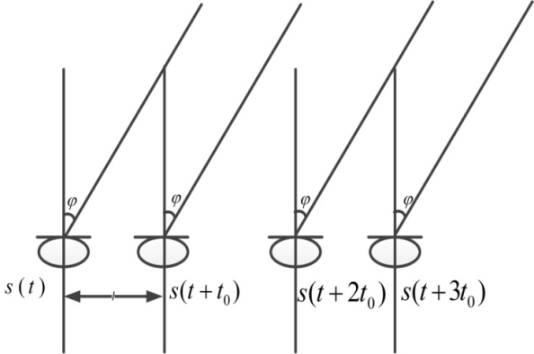 | Figure 1. Estimation of far-field source location. |
 | Figure 2. Estimation of near-field source location. |
 microphone would be[15] Figure. 2:
 | (2) |
 is the distance between source and the first (reference) microphone[15].
3. Feature Selection
- The aim of this section is to compute the feature vectors from the array data and use the MLP (Multi Layer Perceptron) approximation property to map the feature vectors to the corresponding DOA, as shown in Figure. 3.[6].
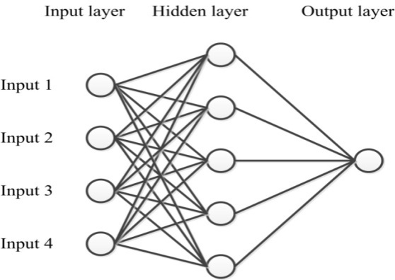 | Figure 3. Multilayer Perceptron neural network for sound source localization. |
 is the signal received at the
  microphone and
  is the reference microphone
 . We can write the signal at the
  microphone in terms of the signal at the first microphone signal as follow:
 | (3) |
 and sensor
  like below:
 | (4) |
 | (5) |
 and
and  to
to  (for
(for ) and thus to the DOA. Therefore our aim is to use an MLP neural network to approximate this mapping.We summarized our algorithm for computing a real-valued feature vector of length (2(M-1)+K)K, for k dominant frequencies and M sensors below:Preprocessing algorithm for computing a real-valued feature vector:1. Calculate the N-point FFT of the signal at each sensor.2. For
  2.1. Find the k FFT coefficients in absolute value for sensor M with compressive sampling.2.2. Multiply the
  FFT coefficient for sensor
  with the conjugate of the FFT coefficient at the same indices for sensor
  to calculate the instantaneous estimate of the cross-power spectrum.2.3. Normalize all the estimates by dividing there absolute values.3. Construct a feature vector that contains the real and imaginary part of cross-power spectrum coefficient and their corresponding FFT indices.We utilized two-layer Perceptron neural network and trained it according to fast back propagation training algorithm[7]. For training network we use a simulated dataset of received signals. We modeled received signal as a sum of cosines with random frequencies and phases. We write received sampled signal at sensor
  as below:
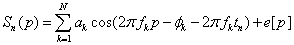 | (6) |
 is the number of cosines (we assumed
 ),
),  is the frequency of the
  cosine,
  is the initial phase of the
  cosine,
  is the time delay between the reference microphone (
 ) and the
  microphone,
  is white Gaussian noise, and
  is uniformly distributed over[200Hz,2000Hz] and
  is uniformly distributed over[0,
 ]. We generate 100 independent sets of 128 sampled vectors, and then calculate feature vectors. A total of 3600 input-output pairs are used to train the MLP.In training step, after making learning dataset and calculating feature vectors, we use compressive sampling algorithm to decrease feature vectors dimension. In testing step for a new received sampled signal, we calculate feature vectors and estimate DOA of sound source. Our experiments show that errors in classification and in approximation have direct relation with number of hidden neurons. Figure. 4 show these relations for far field and near field sources.
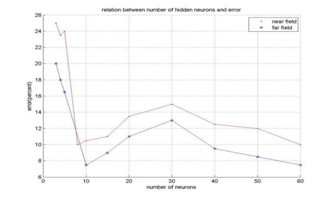 | Figure 4. Relation between number of hidden neurons and error. |
4. Traditional Pruning Algorithms and CS Theory
- Generally speaking, network pruning is often casted as three sub-procedures: (i) define and quantify the saliency for each element in the network; (ii) eliminate the least significant elements; (iii) re-adjust the remaining topology. By this knowledge, the following questions may appear in mind:1) What is the best criterion to describe the saliency, or significance of elements?2) How to eliminate those unimportant elements with minimal increase in error?3) How to make the method converge as fast as possible? Methods for compressing NNs can be classified into two categories: 1) weight pruning, e.g.: Optimal Brain Damage (OBD)[10], Optimal Brain Surgeon (OBS)[4], and Magnitude-based pruning (MAG)[12]. And 2) hidden neuron pruning, e.g.: Skeletonization (SKEL)[8], non-contributing units (NC)[10] and Extended Fourier Amplitude Sensitivity Test (EFAST)[2].A new theory known as Compressed Sensing (CS) has recently emerged that can also be categorized as a type of dimensionality reduction. Like manifold learning, CS is strongly model-based (relying on sparsity in particular). This theory states that for a given degree of residual error ε, CS guarantees the success of recovering the given signal under some conditions from a small number of samples[14]. According to the number of measurement vectors, the CS problem can be sorted into Single-Measurement Vector (SMV) or Multiple-Measurement Vector (MMV). The SMV problem is expressed as follows. Given a measurement sample
 and a dictionary
  (the columns of D are referred to as the atoms), we seek a vector solution
  satisfying:
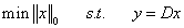 | (7) |
 (known as
  norm), is the number of non-zero coefficient of
 .Several iterative algorithms have been proposed to solve this minimization problem (Greedy Algorithms such as Orthogonal Matching Pursuit (OMP) or Matching Pursuit (MP) and Non-convex local optimization like FOCUSS algorithm[16].
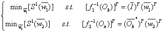
5. Problem Formulation and Methodology
- Before we formulate the problem of network pruning as a compressive sampling problem we introduce some definitions[11, 10]:1. If for all columns of a matrix,
 was smaller than S, then this matrix called a
  matrix.2. If the number of rows that contain nonzero elements in a matrix was smaller than S then this matrix is called a
  matrix.We assume that the training input patterns are stored in a matrix I, and the desired output patterns are stored in a matrix O, then the mathematical model for training of the neural network can be extracted in the form of the following expansion:
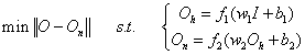 | (8) |
 the output matrix of is neural network,
  is the output matrix of hidden layer
 , are weight matrix of two layers and
  are bias terms.In conclusion, our purpose is to design a neural network with least number of hidden neurons (or weights) that has the minimum increase in error given by
 . When we minimize a weight matrix (
 or
or ), the behaviour acts like setting, in mathematical viewpoint, the relating elements in
  or
or  to zero. Deduction from above shows that the goal of finding the smallest number of weights in NNs within a range of accuracy can consider to be equal to finding an
  Matrix
  or
or . So we can write problem as below:
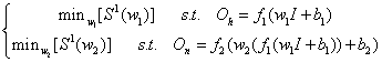 | (9) |
 which most of its rows are zeros. So with definition of
  matrix we can rewrite the problem as below:
 | (10) |
 | (11) |
 | (12) |
 is input matrix of the hidden layer for the compressed neural network. Comparing these equations with 7 we can conclude that these minimization problems can be written as CS problems. In these CS equations
 ,
,  and
and  was used as the dictionary matrixes and
  and
and  are playing the role of the signal matrix. The process of compressing NNs can be regarded as finding different sparse solutions for weight matrix
  or
or .
. 6. Results and Discussion
- As mentioned before, assuming that the received speech signals are modeled with 10 dominant frequencies, we have trained a two layer Perceptron neural network with 128 neurons in hidden layer and trained it with feature vectors that are obtained with CS from the cross-power spectrum of the received microphone signals. After computing network weights we tried to compress network with our algorithms.In order to compare our results with the previous algorithms we have use SNNS (SNNS is a simulator for NNs which is available at[19]). All of the traditional algorithms, such as Optimal Brain Damage (OBD)[16], Optimal Brain Surgeon (OBS)[17], and Magnitude-based pruning (MAG)[18], Skeletonization (SKEL)[6], non-contributing units (NC)[7] and Extended Fourier Amplitude Sensitivity Test (EFAST)[13], are available in SNNS (CSS1 is name of algorithm that uses SMV for sparse representation and CSS2 is another technique that uses MMV for sparse representation).Table 1 and 2 demonstrate the results of the simulations. Observing these results, in table I we compare algorithms on classification problem and in Table 2 we compare algorithms on approximation problem. For classification problem we compare sum of hidden neurons weights in different algorithms with similar stopping rule in training neural networks. Another thing that we compared in this table was classification error and time of training epochs. In Table 2 we compare number of hidden neurons and error in approximation and time of training epochs, where we have stopping rule in training neural networks. With these outputs we can infer that CS algorithms are faster than other algorithms and have smaller error in compare with other algorithms. In comparison to other algorithms CSS1 is faster than CSS2 and would achieve smaller computational complexity. This means that, According to the number of Measurement vectors, the algorithm that uses single-measurement vector (SMV) is faster than another algorithm that uses multiple-measurement vector (MMV) but its achieve error is not smaller.
|
7. Conclusions
- In this paper, compressive sampling is utilized to designing NNs. Particularly, using the pursuit and greedy methods in CS, a compressing methods for NNs has been presented. The key difference between our algorithm and previous techniques is that we focus on the remaining elements of neural networks; our method has a quick convergence. The simulation results, demonstrates that our algorithm is an effective alternative to traditional methods in terms of accuracy and computational complexity. Results revealed this fact that the proposed algorithm could decrease the computational complexity while the performance is increased.
References
| [1] | R. Reed, "Pruning algorithms-a survey", IEEE Transactions on Neural Networks, vol. 4, pp. 740-747, May, 1993 |
| [2] | P. Lauret, E. Fock, T. A. Mara, "A node pruning algorithm based on a Fourier amplitude sensitivity test method", IEEE Transactions on Neural Networks, vol. 17, pp. 273-293, March, 2006 |
| [3] | B. Hassibi and D. G. Stork, "Second-order derivatives for network pruning: optimal brain surgeon," Advances in Neural Information Processing Systems, vol. 5, pp. 164-171, 1993 |
| [4] | L. Preehcit, I. Proben, A set of neural networks benchmark problems and benchmarking rules. University Karlsruher, Gerrnany, Teeh. Rep, 21/94, 2004 |
| [5] | M. Hagiwara, "Removal of hidden units and weights for back propagation networks," Proceeding IEEE International Joint Conference on Neural Network, vol. 1, pp. 351-354, Aug. 2002 |
| [6] | M Zhou Yan; Wu Xia, "Quantum Neural Network Algorithm Based on Multi-agent in Target Fusion Recognition System," Computational and Information Sciences (ICCIS), Dec, 2010 |
| [7] | Zhaozhao Zhang; Junfei Qiao, "A node pruning algorithm for feedforward neural network based on neural complexity," ICICIP, Aug, 2010 |
| [8] | E. J. Candes, J. Rombcrg, T. Tao, "Robust uncertainty principles: exact signal reconstruction from highly incomplete frequency information," IEEE Transactions on Information Theory, vol. 52, pp. 489-509, Jan. 2006. |
| [9] | J. Haupt, R. Nowak, "Signal reconstruction from noisy random projections," IEEE Transaction on Information Theory, vol. 52, pp. 4036-4048, Aug. 2006 |
| [10] | Y. H. Liu, S. W. Luo, A. J. Li, "Information geometry on pruning of neural network," International Conference on Machine Learning and Cybernetics, Shanghai, Aug. 2004 |
| [11] | J. Yang, A. Bouzerdoum, S. L. Phung, "A neural network pruning approach based on compressive sampling," Proceedings of International Joint Conference on Neural Networks, pp. 3428-3435, New Jersey, USA, Jun. 2009 |
| [12] | H. Rauhut, K. Sehnass, P. Vandergheynst, "Compressed sensing and redundant dictionaries," IEEE Transaction on Information Theory, vol. 54, pp. 2210-2219, May. 2008 |
| [13] | T. Xu and W. Wang, "A compressed sensing approach for underdetermined blind audio source separation with sparse representation," 2009 |
| [14] | J. Laurent, P. Yand, and P. Vandergheynst, "Compressed sensing: when sparsity meets sampling," Feb. 2010 |
| [15] | G. Arslan, F. A. Sakarya, B. L. Evans, "Speaker localization for far field and near field wideband sources using neural networks," Proc. IEEE-EURASIP Workshop on Nonlinear Signal and Image Processing, vol. 2, pp. 569-573, Antalya, Turkey, Jun. 1999 |
| [16] | Yang Geng; Jongdae Jung; Donggug Seol, Sch. of Inf. Technol., Korea Univ. of Technol. & Educ., Cheonan, " Sound-source localization system based on neural network for mobile robots", IJCNN, JUN 2008 |
| [17] | B. Hassibi and D. G. Stork, "Second-order derivatives for network pruning: optimal brain surgeon,” Advances in Neural Information Processing Systems, vol. 5, pp. 164-171, 1993 |
| [18] | M. Hagiwara, "Removal of hidden units and weights for back propagation networks," Proc. IEEE Int. Joint Conf. Neural Network, pp. 351-354, 1993 |
| [19] | S. H. Chagas, L. L. de. Oliveira, J. Baptista, S. Martins, "Review of Localization Schemes Using Artificial Neural Networks in Wireless Sensor Networks", 26th South Symposium on Microelectronics, april 2011 |
| [20] | SNNS software, available at http://www.ra.cs.unituebingen.de/SNNS |