1. Introduction

The vehicle population in the Republic of Mauritius is 574,772.00 [38], that is 45% of the population, which is 1,265,711 [40]. These demographics clearly show that the vehicle to person ratio on the island is high at 1:2.2 compared to many developing countries on the African continent, such as Liberia 1:3.9, Nigeria 1:12, South Africa1:5 and Tanzania 1:47 [39]. On one end, this echoes prosperity as members of the community have easy access to services that require vehicles. However, on the other hand, this raises concerns about the environment. Mauritius being an island state, a part of non-continental Africa, a tropical heaven in the Indian ocean, which derives a great measure of its wealth from the tourism industry, would do well to comply to national and international protocols on environment protection.

Given that Mauritius is a signatory to numerous conventions on environment protection, it has an obligation to assess the impact of the disposal of Used Lead Acid Batteries (ULABs). The Basel Convention classifies ULABs as hazardous waste [21] Years of importation of vehicles, result in a large population of vehicles, this in turn, results in many parts which are disposed of in the environment, among which are vehicle batteries.

17,000–18,000 tons of Hazardous Wastes (HW) are generated annually [12], of these ULABs constitute 1100 tons. The annual 1100 tons of ULABs that are generated each year are a very dangerous health risk to the community and the environment if they are not safely collected and properly disposed. A long distance to collection facilities increases the risk of spillage or leakage to the environment and increases the risks associated with long term storage. If there is no ULAB collection facility nearby, users store the dangerous waste in their garage, or in the back yard for the whole year, where children might play with the harmful ULABs.

Section 75(1) of the Environmental Protection (Hazardous Waste Standards) Regulations 2001 of the Environmental Protection Act 1991 of the Republic of Mauritius, provides that no individual shall use, store, transport or otherwise deal with hazardous waste except when that hazardous waste is stored in a container or package - (a) built and constructed to prevent spillage or leakage into the environment (b) materials from which the waste is not susceptible to attack or which are liable to form harmful compounds with the waste; and (c) materials from which the waste is not susceptible to attack; and (d) materials designed to ensure safe, full or partial emptying of the waste [15]. The law has provisions to ensure the safety of the environment and reduces the pollution that results from the handling of all hazardous waste, including ULABs. However, the absence of an appropriate collection system does not help in the enforcement of the regulation.

The atrocious dangers and the adverse health problems associated with ULABs developed the need to study where and how they are being disposed of, in the Republic of Mauritius, to reduce or eliminate the contamination of the environment, and to avoid the harmful health effects associated with lead exposure.

Thus, the following objectives were formulated for this research study:

1. To investigate the disposal of ULABs in Mauritius.

2. To investigate the impact of the disposal of ULABs on the Mauritian environment.

3. To model the collection of ULABs for the purpose of exportation.

4. To develop a model of reverse logistics that utilizes the k-median problem to locate collection points for ULABs.

2. Literature Review

2.1. The Impacts of Lead Exposure from ULABS in the Republic of Mauritius

A survey conducted [17] evaluated the lead burden of the Mauritian population. A sample of 312 people were chosen as selected occupational and residential subgroups. Blood samples from these individuals showed a high blood lead in certain population groups in Mauritius, such as traffic policemen, paint sprayers and petrol station attendants, with levels averaging 12-15 mcg dl ^(-1) [17].

High blood lead results were detected in the vicinity of a lead battery factory on the outskirts of the capital city Port Louis in which 4 children living adjacent to the battery factory were found to have blood lead in the range 30-66 mcg dl ^(-1) [17]. This research was conducted in the early nineties; however, the survey proved the dangers that some members of the population were facing due to the ULAB contamination then. 30-66 mcg dl ^(-1) is very high and at a level harmful to the developing brain of young children. Since [17] there is a wide gap in research and not much data on the subject. Journal articles and reports on this danger are scarce.

2.2. k-median Problem

When it comes to solving economic decision problems that involve the accurate siting of facilities to serve a given set of demands efficiently, the k-median objective function has been considered a better objective function than the mean or the center because of its robustness or its resistance to outliers. [1]. The k-median algorithm is a variant of the k-means clustering technique. The aim of the K-means algorithm is to minimize the sum of squared distances between the data points and their respective cluster centroid. The data collected in many real-world applications may be contaminated with outliers, which can make traditional clustering methods such as K-means sensitive to their presence. Thus, robust clustering algorithms such as k-medians are used to produce more reliable outcomes [2].

Clustering is a popular form of unsupervised learning for geometric data. [3]. Unsupervised learning deals with unlabeled data, neither an example is given to the model, nor an output is given; only input data is given and based on that the model makes predictions. [13]. k-Median is perhaps the most well-studied clustering objective in finite general metrics. [19] In metric k-median clustering, we are given as input a set of n points in a general metric space, and we have to pick k centers (geometric medians) and cluster the input points around these chosen centers, so as to minimize the median objective function [13].

The objective of the k-median algorithm is to decide the optimal locations to locate collection facilities to serve the clients who are, in this case, the population with used-up or failed vehicle batteries in Mauritius. A hard limit is provided for the exact number of facilities opened in the k-median problem, which is an upper bound k this is different from the Uncapacitated Facility Location Problem (UFL), where the cost of opening a facility and the cost of linking customers to that facility is given. With the k-median problem there is no opening cost of the facilities and there is a numbered limit represented by k, of the maximum number of facilities that can be opened.

It also differs from the p-median problem which is forced to open exactly p facilities. In the k-median problem, k is the maximum number limit of facilities can be open in the final solution. A k-median solution may open less facilities than the k number given, but a p-median solution is forced to open the exact number given for p. They both, however, seek to minimize the distances from each client to the median located facility surrounded by all the clients closer to the open facility.

The k-median problem is mainly used when the opening costs of facilities are uniform, trivial, negligible and not significant enough to include in the decision of optimal locations for facilities. In this study a green earth organization offered to build the collection facilities for free thus removing the burden of the cost of opening the facilities thus the remaining decision was to establish the optimum locations to site the ULAB collection facilities.

Figure 1. k-median-instance

The k-median problem becomes: the need to place a given number k, of used-up or failed vehicle battery collection points on the island Mauritius. Where should the given number of k collection points be located, so that the average travelling distance of people with used-up or failed vehicle batteries to the nearest collection point is minimized. Assuming there is a limited budget to build only k collection points. The aim is to optimally choose the collection points of k to minimize the overall collection costs and to minimize the distance for customers to motivate them to carry the batteries used to the collection points located nearby.

A set of possible locations of the facilities , is a set of potential collection points for used or failed vehicle batteries, the set of clients, is a set of people with used or failed vehicle batteries which need to be sent to the nearest collection center to be recovered or replaced or recycled, and finally the X data set, is a data set of all the potential collection facility locations and client locations that need to be partitioned into k clusters.

If [13]

partitions a set of geometric points into clusters, the objective function of the k-median algorithm thus measures how well the X data set can be partitioned into k clusters.

Thus, the dataset X contains the whole set of facilities and the whole set of clients combined. While is the subset of that consists of the optimum set facilties to be opened out of the whole set of facilities , these characterise the solution set. While the modulus of these optimum set of facilities is the upper bound k which is the limit on the number of facilities which are required to be opened, thus the solution set of facilities opened at the given number of k facilities.

The Euclidean distance metric is used to solve the k-median problem in this thesis which is also known as the 2-norm distance. This direct line distance is a generalization of the Pythagorean theorem to more than two coordinates. If a straight line calculates the distance between two points, the Euclidean distance or direct line distance is obtained. This is the most common distance measure and, in this case, the most available.

2.2.1. Notations

i is used to denote a potential facility location. A potential facility location is a location on which a facility can be located to achieve an optimum cost and an efficient distribution of the facility’s resources.

j is used to denote a client. A client is the area which needs or requires the services of a nearby facility. It can be a city, region, a society or an individual customer.

x_ij is a decision variable which denotes whether facility i is connected to client j or not. x_ij is a binary variable, which becomes 1 if facility i is connected to client j or 0 if facility i is not connected. Being connected means the client receives its services from the open facility.

y_i is a decision variable which denotes whether facility i is open or not. y_i is a binary variable, which becomes 1 if facility i is open to receive clients or 0 if facility i is not open.

d_ij denotes the distance from client j to facility i. The distance determines the cost which must be minimized. The distance is only a significant cost if the facility i is open and connected to client j, that is if x_ij is 1.

F is the larger set of potential facility locations. The goal is to open the best located set of facilities, which serve all the clients with a minimum cost. The best located set of facilities is chosen and opened from the larger set of potential facility locations. There is the choice to select the best located, open them, and let the rest remain closed.

C is the set of clients. All the clients must be served. All the clients must be connected to its closest open facility. Unlike facilities where there is a choice to select the optimum located, open them, and let the rest remain closed.

F’ is the set of open facilities. This is when the best set of facilities is chosen and opened from the larger set of potential facility locations.

k is a limit or an upper bound to the number of facilities that can be opened.

2.2.2. Mathematical Formulation of the k-median Problem

A major advantage of the integer programming formulation of the k-median problem is that most ecosystems for scientific computing offer different solvers for linear and nonlinear integer programs [11].

The formulation of the metric k-median problem as an integer program proposed by [11] is the same as equation 1-5:

(1)

Subject to the constraints:

(2)

(3)

(4)

(5)

(6)

The scope of the k-median problem for this study is nationwide, the ULABs need to be safely collected from everywhere in the republic of Mauritius. There is a need to optimally locate ULAB collection facilities efficiently near all the potential clients who would want to dispose them. The reason is to cover all the clients efficiently. Due to the complexity and the combinatorial nature of the k-median problem, the problem is NP-hard which implies that if P≠NP there is no algorithm known, which can find an optimal solution in polynomial time.

2.3. The Gap is in the Real-World Application of the k-median Algorithm

The gap in existing literature is in the real-world application of the theoretical k-median algorithm. Many of the k-median algorithms have not yet been applied to realistic, real-world scenarios. The real-world application has multiple factors that might alter the approximation factors of these algorithms per instance. The main reason for solving the k-median problem is to serve a set of clients or cities by opening facilities in optimum locations, the optimum locations being those that achieve a minimum cost at serving all the clients.

To the best of our knowledge all known prior methods are targeted to achieve the fastest, most efficient, and optimal method of solving the computationally intractable k-median problem, were using a distance matrix as data input in their calculation. In this study we eliminate the use of this distance matrix.

However, as close to the approximability lower bound [8] of the k-median problem prior algorithms may have achieved, which is approximately the closest level ever possible to an optimum solution, practical examples are missing and still needed for the real-world application of these algorithms. Case studies in this field are scarce and very rare.

Instance creation is somewhat easy when instances are created artificially, or when they are generated randomly using software. However, when this is done on a practical scenario, a lot of unforeseen complications may unravel. The algorithms are effective when they are applied to an instance which has already been created, the bipartite graph G with bipartition (, ), where is the set of facilities and is the set of cities [8]. However, in the real world this instance is not yet created. This could be one of the most time-consuming and complex steps in solving this problem practically.

Cases in which these algorithms have been used to solve real world problems, and in which they have been analyzed confronting the real challenges in the world and achieving satisfying results that prove their guarantees are missing. The application of these algorithms in a real-world setting will achieve more in terms of revealing the limitations and boundaries of the algorithms. When they are analyzed from the basis of reality a further extension of the qualities of the algorithms may give way, and be revealed, this gives a chance for modifications and improvement.

When solving the problems practically the instance has got to be created, and for the algorithms to work on the instance, the instance would have to fit the model and the assumptions under which the algorithm was developed. This could give rise to cases were an instance might be too complex to develop accurately to solve the problem. The choice of data which constitutes the set of facilities and the data which constitutes the set of clients in a real-world environment must be carefully determined from multiple possible of choices to accurately solve the problem. The worst-case analysis might prove to have an even worse case where an instance cannot be created for the specific case, thus the need for worked solutions. Appendix C to E displays the journey that was taken to create the right instance using ArcGIS.

2.4. Contribution of the Euclidean Distance Formular to the k-median Problem in CPLEX Opl

To the best of our knowledge, all known prior algorithms use the input of a distance matrix, as input in the calculation [22]. The removal of the distance-matrix in the calculation is the main difference between the model solution developed to solve the k-median problem in this case, and all known prior methods of solving this problem. For example, [5] use the distance matrix below (a), in a small nine warehouse example. Even in their short example, to ensure that the distance of each point to the other remaining eight points is combinatorically considered, is a big combinatorial task. This becomes even more complex when you must gather the data between all possible combinations of distances, for example if there are 50 locations : From the first location we label it L 1 to the last location L 50

L 50 ->2⁴⁹ lists all the possible pairs

L 49 -> 2⁴⁸ lists all possible pairs (same as above, excluding L 50)

2⁴⁹+2⁴⁸+…+2⁰=2⁵⁰–1

Continue with this to the last location L1 then add them up we have 1.1258999e+15 location distances to place in a distance matrix. This is somewhat easy when it is randomly generated by software, however, in real world practice this is extremely complex [22]. Below is a distance matrix of only 9 locations.

(a)

This would be impractical in many cases in the real world where there might be hundreds or thousands of location points, and the distances that make each pair of distances. Thus, a new model is developed that does not need the input of the distance matrix but uses the formular for the Euclidean distance between two points and the input of actual GPS coordinate location points to solve the k-median problem.

The formular for the Euclidean distance between two points is:

(b)

The k-median Cplex Opl Euclidean distance formular developed for this study

(c)

(d)

The new method solves the k-median problem by making a choice between facility locations and client locations, without considering the distance between all the points as a distance matrix [22]. The newly developed method only requires the GPS coordinate location points. This means that it opens the best out of n potential facility locations and assigns only m clients to these open facilities per calculation. It is a heuristic solution technique, an Integer binary linear program with binary variables that solve the k-median problem. The new method could also be a useful contribution in k-median approximation algorithms, where it could contribute to a faster approximation algorithm for the k-median problem.

3. Methodology

To achieve the first two objectives, quantitative research, which sought to describe the existing structure and network of the ULAB life cycle, from the importation to the disposal was chosen. Numbered data was analysed using statistical procedures and techniques. The results showed that 55% of the respondents strongly agreed that there is a need to develop a new collection system. Survey research was conducted which involved raw data collection and statistical analysis on published health data from the Mauritius Institute of Health and Metrics Evaluation.

There were also some qualitative findings from the face-to-face interviews, which were compared and analysed. An unsafe, market controlled, nationwide, yearly collection system was found to be in place and mentioned by many respondents to the survey. Respondents strongly agreed that the collection system in place is not safe and risks the lives of the employees collecting them and their families. The public is also at risk from the yearly in-house storage before the collection and exportation. Members of this industry disclosed that the public is not informed of the dangers of this industry, thus there is a lack of public awareness.

During face-to-face interviews and in the questionnaires, many members of the automotive industry and those of the health industry disclosed the need of a new and a safer system for the collection of ULABs. The first two objectives of this study established the mandatory need to model a new and a safer system for the collection of ULABs in the republic of Mauritius. ULAB collection points being a type of facility, the third and fourth objectives of this study sought to model the collection of ULABs for the purpose of exportation, and “more specifically” to develop a model of reverse logistics that utilizes the Uncapacitated facility location k-median problem to locate collection points for ULABs.

3.1. Mathematical Formulation of the New Solution k-median Model

Prior work on the Travelling Salesman Problem (TSP) Opl model by [4], and the p-median problem Opl model by [5] was combined, modified, and reconstructed to invent a new k-median software model. An experimental software analysis of [4] revealed the similarity in the objective functions and the constraints of the TSP, p-median and k-median problems. This lead to a deeper analysis of the objective functions and the constraints of these three problems in the CPLEX Opl programming language. The formulation of the equations 1-16 show changes that were made to the TSP and p-median formulation to develop a k-median formulation in CPLEX Opl which combined the two formulations. This eliminated the subtour elimination constraint of the TSP and changed the non-negativity constraints. However, the functionality of the TSP by [4], which required the use of the Euclidean distance formular was then usable when solving the k-median problem.

The mathematical formulation of the TSP problem, as cited from [4] is:

(6)

(7)

Subject to the constraints:

(8)

(9)

(10)

In general, the objective of the k-median equation (eq1) involves the summation of the total distances, from each client to the open facility nearer to it.The TSP equation (eq7) only carries the summation of the distances from one j client to the nearest client i.

Thus, for the TSP, the medium equation of the lower limit of the summation of the distances must specify that the starting point _j is a client but is not the same as or is not equal to the ending point client i. Otherwise, that would be the shortest distance from j to i on the same point. Thus, it is specified in the lower limit of the summation of the TSP objective as **(j≠i). The removal of this equation in the CPLEX Opl code is a first step when converting a TSP algorithm to k-median algorithm.

In the objective function of the k-median equation (eq1) there are two separate sets of location points where is an element of the set of Facilities and is an element of the set of client location points While for the TSP problem (eq7) there is only one containing set of location points where is an element of the set of start points location for the path of an edge and is an element of the set of the end point locations of an edge.

These are all contained in the same set of locations however in an iteration the same location picked for the beginning point of an edge, node or path cannot be the same location picked for an ending point of the same edge at the same time, there would be no distance, “zero distance” because it starts where it ends**(j≠i). Thus, the objective is to derive the shortest possible distance that runs through all the locations from all the edge distances, these being in the same set.

The observations above lead to an experiment in which the Location set A, of the TSP by [4], in which was separated into two arrays that conform to the k-median problem. Location sets and in which are on Figure 2 renamed to ulabfacilitylocation for while the array is labeled ulabcitylocation.

The first constraint of the k-median problem (eq2), which states that every client must be connected to a facility, is comparable to the first constraint of the TSP (eq8) which states that every starting point location must be connected to an ending point location. From the similarity and the prior changes made to the sets of location points, it is possible to convert these constraints to the other in the CPLEX Opl language.

The second constraint of the k-median problem (eq3), which states that every client must be connected to an open facility, is comparable to the second constraint of the TSP (eq9) which states that every ending point location must be connected to a starting point location which simply reverses the same connection as the first connection. Thus, for the TSP every starting location point in the set must be connected to its closest location ending point while each location ending point must be connected to a starting point through all the locations in the set.

The TSP subtour elimination constraint (eq10) is completely removed when converting an algorithm to the k-median problem because it is not relevant or applicable in this case. Thus, remaining only, the non-negativity constraints (eq4) and (eq5) can be included.

The similarity in the calculation is that both the k-median and TSP seek to minimize the distance between location points. Thus, from the similarity and the prior changes made to the sets of location points, it is possible to convert these constraints either way as algorithms in the CPLEX Opl language. Arrays of the facility locations and opening costs were added, these enabled the costs of the edges to be computed from each facility to each client. The changes have developed an entirely new software solution to the UFL problem.

The mathematical formulation of the p-median problem is [5]:

(11)

Subject to the constraints:

(12)

(13)

(14)

(15)

(16)

In the objective of the p-median problem equation (eq11) there are two separate sets of location points where is an element of the set of Facilities and is an element of the set of client location points . Thus, the objective of the p-median problem equation (eq11) and that of the k-median problem equation (eq1) are identical in that respect. The p-median (eq11) considers summation of the total distances from each client to a facility nearer to it.

However, in this special case (eq11) by [5] they include the demand from each client. The demand in the case of ULABs is unknown as this is the first time that this project is proposed hence in this case it is irrelevant, hence it is removed from the objective of the p-median in CPLEX Opl. Thus, the remaining are the variables are which calculate the total distances from each client to a facility nearest to it, and the decision variable which indicates if a facility is open or not.

The first constraint of the k-median problem (eq2), which states that every client must be connected to at least 1 facility, is comparable to the first constraint (eq12) for p-median which also states that every client must be connected to a facility. The second constraint of the k-median problem (eq3), which states that every client must be connected to an open facility, is comparable to the second constraint (eq14) of the p-median which states the same. They are identical in that if a client is connected to a facility the decision variable then that facility must only be open Thus, in both cases the client cannot connect to a closed facility because a facility only opens if it is in the minimized solution set of facilities.

The remaining constraint for the p-median equation (eq13) compares to the k-median constraint (eq 4). The inequality in (eq4) proves their difference where for the k-median it means it can open less than or equal to k facilities. While this constraint (eq13) forces the p-median to open exactly p number of facilities as shown by the equal’s sign. Thus, a solution can be developed which combines the p-median and the TSP problem solution algorithms developed in CPLEX Opl and converts part of their code to produce a k-median problem solution.

The p-median constraints where then modified to suit the k-median constraints as shown in Appendix A. Appendix A shows the newly developed algorithm that draws from the data file on Figure 2.

3.2. The ESMVERE Cplex k-median Model

This section tests this solution for accuracy and efficiency in locating facilities, or in the design of a facilities network. To test the solution model for accuracy, an instance of the k-median problem, a diagram was used, Figure 1. The x and y coordinates of the clients and facilities were plotted and measured on all the points on plane to produce the data on the diagram Figure 2 which shows the arrays of these coordinates. The instance hosts 7 potential facility locations and 21 clients.

However, in this case it is now used again to compute the solution to the data instance diagram as Figure 2. The potential facilities in this example diagram are read from the left to the right as facilities 1,2,3,4,5,6 and 7. The clients, also called the cities or in this case called the (ulabcities), are displayed on the diagram as small dots. The clients are also read from the left to the right; however, they are 21 clients that are identifiable with their x and y coordinates.

The diagram, Figure 2 displays the CPLEX data file, which contains the data values which have been input manually to test the application. The value of the number of (ulabfacilities) is 7 in the test case, and the value of the number of ulabcities is 21 in this test case. The value of on this diagram is given as 6 this is just as an example on this diagram. The other diagrams display a solution for k as 6. It also contains the values of the two arrays, ulabcityLocation and ulabfacilityLocation which host the and coordinates of ulabcity locations and ulab collection facility locations. To develop the test coordinates an x axis and a y axis were placed on a printed copy of the diagram using a 30-centimeter ruler.

It also contains the value of in which is the input of the limit of ulab collection facilities. The objective of the k-median problem only considers minimizing the average sum of distances from each (ulab city) to its nearest open (ulab collection facility). The last constraint is a k-median constraint that places a limit on the number of facilities to be opened.

If one only considers the distance from a facility to a city and one tries to minimize the total distance without considering the cost of opening a facility, then the more facilities one has, the better, the objective value. With more facilities, there are more chances for the cities to find a facility closer to them. The answer is the more facilities there are, the better. If there are maximum 7 facilities, then the answer for the best k is 7, If there are 20, then the answer is 20. Because there are no costs for opening the facilities, the main reason is to establish the locations which are the median facility.

Thus Figure 2 is the data file for input of data.

Figure 2. Prototype data

Diagram Figure 3 displays the solution to the decision variable . After running the data on Figure 2 in the CPLEX Optimization Engine, the solutions to the decision variables are displayed as on Figure 3. On the left half side of the diagram the CPLEX Engine displays a Solution with objective 45.043, this is the minimum cost solution of the k-median Problem calculation please note it also displays the input value of k as 6.

The minimum TotalDistance of 45.043 centimeters. The solution to the decision variable is displayed on the right half of the diagram Figure 3. This side displays a list of all the edges This displays edges (size147), meaning in combination there are 147 edges between the facilities and the clients.

Figure 3. Variable x

Thus, from all the possible combinations of edges, after the calculation, the least cost edges, edges that give a minimum distance when connected to clients, are displayed with Boolean values of 1, while connected to the open facility. The edges which are connected to open facilities have Boolean values 1 and those not connected display Boolean values 0. Figure 3 displays how the cities 3,4 and 5 are connected to the open ulabfacility 1. All the cities in the solution are connected to the 6 open facilities, which are all the facilities except facility 3 displayed with a 0.

The diagram Figure 4 displays the solution to the decision variable . The solution to the decision variable is displayed on the left half of the diagram Figure 4 as an array with seven numbers or seven locations . Thus is a boolean decision variable, which places a 1 on an open facility and a 0 on a closed facility. Thus, the solution in Figure 4 opens the ulabfacility locations 1,2,4,5,6 and 7.

Figure 4. Variable y

The solution to the decision variable is also displayed on the right half of the diagram Figure 4. This side displays a list of all the facilities , this displays ulabfacilities(size7), meaning there are 7 facilities listed down from facility 1 down to facility 7. The corresponding boolean value of the facility is displayed to the right side as either a 0 or a 1, for a closed or open facility respectively.

The right half of the diagram Figure 5 displays the list of each edge, this displays edges(size147) and its value value in terms of its size or distance to the facility it is connected to. This is a list of all the possible combinations of distances from the ulabcities to the ulabfacilities.

Figure 5. Cost of each edge

This value is critical in the calculation of the distances, to the point of the selection of the minimized cost set of distances from the clients to the facilities, which then results in the solution of which set of facilities to open. This is a very high level of accuracy as also evidenced by the values of each edge given on the diagram Figure 5.

4. Results and Discussions

This chapter gives evidence of the usefulness of the newly developed software model. The model is used in the real world, on a practical case to develop the ULAB collection network in the republic of Mauritius. The solution proves how it guides management in selecting the optimum locations to place the ULAB collection facilities, while minimizing all the costs and distances.

4.1. Results

4.1.1. Sensitivity Analysis

The performance of the ESMVERE Cplex k-median is compared with [37] on a simulation study in terms of computation speed and accuracy of the estimations, with more classical partitioning techniques such as k-means, trimmed k-means and PAM (partitioning around medoids [37]. The MacQueen [36] set of instances were used to test the algorithm in large international test cases. Mean computation times, for 100 runs, various sample sizes and numbers of clusters are reported on the tables below

A comparison of the mean computation time in seconds, for 100 runs of the different algorithms for various sample sizes n =250,n=500and n=2000 and number of clusters k. The computation time is given for one initialization point [37].

Table 1

The MED set of instances from [16] [1] [3] [23] are compared and used to analyze the quality and performance of the ESMvere k-median algorithm on the larger cases. The sets contain 18 large-scale problems used by [3] in the context of p-median. IBM ILOG CPLEX Optimization Studio 22.1.2 Developer Edition was to test and compare the performance of the algorithm in larger instances. This enabled the algorithm to solve larger instances of sizes, up-to 1000 facilities and 3000 clients.

ESMVERE CPLEX k-median compared to the MED set of instances [23].

Table 2

In the larger instance experiments are given the CPU-times for the ESMvere CPLEX k-median. Columns optt stands for the CPU-time needed to find the best solution in the execution and, Column time stands for the full CPU-time of the execution [3]. Compared to ILS, MDAS, HYB the ESMvere CPLEX k-median method finds better solutions to all problem instances and requires smaller average CPU-time in all the cases. This has proved the effects of removing the distance matrix, the ESMvere CPLEX k-median algorithm has shorter running time.

ESMvere Cplexk-median best solutions compared to the ILS, Gurobi best solutions for MED test problems [3].

Table 3

The ESMvere CPLEX k-median obtains higher quality best solutions for all MED instances. A thorough emphasis was also placed on the instance creation process in the real world and the accuracy of the algorithms in solving the single instance created for the problem. Cases of this are rare or missing in literature.

4.2. Implementation Results

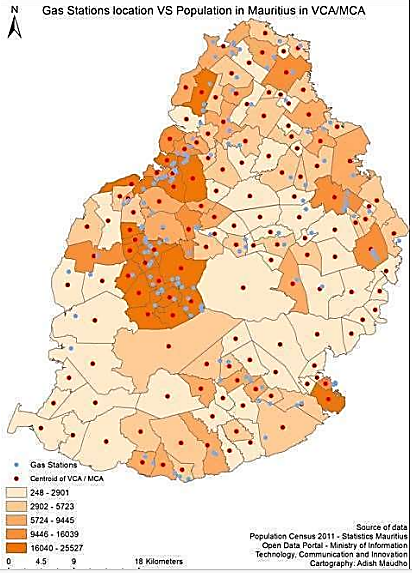
For a company that is in the business of recycling or exporting ULABs, the optimum locations for them to place ULAB collection facilities, could be given as a map with triangles and dots (Figure 6), or a list of geographic coordinate points. The map and the list give the optimum locations to open all the ULAB collection facilities, to have an optimum least cost ULAB collection network. The map and the list of coordinate points were established, and the calculation of the model returned nineteen optimum locations according to the k-median problem. The 19 locations were chosen by k=2 for 2 facilities in each region for 8 regions of the 9 regions, thus 16 facilities, then for the most populated Port Louis region k=3.

The nineteen optimum locations are listed in the following sections according to their districts. The 152 gas stations in the whole Republic of Mauritius [8], were all considered as potential facility locations. The optimum set F’, out of the whole 152 gas stations (ulab collection facilities) was calculated against the 144 (ulab cities).

The goal was to develop a minimum cost reverse logistics network, hence the computation of the models left out some locations and picked up some locations from the large set F of 152 potential facility locations, to the optimal F’ of nineteen facilities which was calculated by the ESMvere CPLEX k-median Solver Model. The nineteen coordinate points can be tested, they can be input on ArcGIS (Figure 6) or Google Maps to verify the accuracy of the solution visually.

The centroid of each district (red dots Figure 6) was taken to be the client location, these together were 144. However, because of the magnitude or size of the calculation (152x144) and since it is a computationally intractable combinatorial problem, the data was partitioned into regions.

Thus, the whole map of Mauritius was divided into 9 districts namely Port Louis, Pamplemousses, Riviere du Rempart, Flacq, Grand Port, Savanne, Plaine Wilhems and Moka districts. Thus, the coordinates of the Gas stations in each of the 9 districts were calculated against the coordinates of the clients in each district.

Figure 6 shows the ArcGIS display of the optimum ULAB collection network. The network considers and minimizes the opening costs of the facilities as well as the distances from all clients to the lowest-cost facility opened and minimum distance to opened facilities network.

The pattern of the opened facilities in the solution appears accurate in terms of how it opens facilities that are in the median of all the client points in the district. By mere observation, it is visible that most facilities being opened are in the median center of the district for all the clients displayed on the map.

Figure 6 shows the final near optimum solution which hosts nineteen facilities.

Figure 6. k-median Optimum Solution [14]

5. Conclusions

A model of reverse logistics that utilizes the ESMvere Cplex k-median problem to locate collection points for ULABs was simulated and designed to accommodate nineteen ULAB collection points. The nineteen coordinate points can be tested, they can be input on google maps to verify the accuracy of the solution visually. The location solutions were tested using ArcGIS and google maps. The results were sound in that they gave truthful real live coordinates of the best locations, the minimum cost locations Figure 6 which were located generally at the minimized distance and cost locations.

The solutions developed in this study are all usable in other industries and for other purposes besides the purpose of this study. This is because the models are separated from the data. A simulation solution was developed that helps in the safe collection and disposal of ULABs. A reverse logistics network was modeled that has the coordinate points of the nineteen optimum locations to establish the collection facilities for ULABs.

Conflicts of Interest

The authors declare no conflicts of interest regarding the publication of this paper.

Appendices

Appendix A

The ESMvere CPLEX k-median Problem Solver Model

The ESMvere CPLEX k-median problem solver algorithm is a software invention that solves the k-median problem. It is a tool that aids, and guides management in making sound decisions on where to locate facilities. It aids management in the decision of where the best places are, lowest cost places, the minimum distance places to locate facilities considering that there are no opening costs and the Euclidean distances, direct line distances of GPS coordinate points?

The CPLEX Opl Code

Appendix B

The ESMvere CPLEX k-median Solution Model test demonstration.

Out of 144 client locations, 125 locations were selected from the Northen densely populated areas, whereas 19 client locations were dropped from the southwest, spacey populated areas.

The 152 potential facility locations were computed making a choice of the best locations within each region, using the same set of clients. The ESMvere CPLEX k-median solution model in this case computed the solution by partitioning the whole map of Mauritius into regions. Densely populated regions such as Port Louis were computed first.

The division of the whole Republic of Mauritius map into regions was sensible and effective in that some regions to the southwest of Mauritius are too spacey populated, thus in these regions it would be more feasible to open all the ulab collection facilities. Whereas in areas that are too densely populated it would be more effective selecting the few facilities that would serve all clients with a minimum cost.

The other method which was adopted as the more efficient and accurate method, was to divide the whole country of Mauritius into districts. The division of clients and facilities into districts meant that the calculation would be more accurate as it would be between the facilities and the clients that are in that district. In this method the computation to establish the optimum network would again, must be computed in series.

The capital city Port Louis has a total of 17 gas stations. The company Total service stations own 7 gas stations, whereas the company Shell service stations also own 7 gas stations, 2 gas stations belong to Engen and 1 gas station belongs to Indian Oil. Figure 7 displays the solution to the decision variable . The solution to the decision variable is displayed on the left half of the diagram Figure 7 as an array with seven numbers or seven locations .

Figure 7. Total Gas in Port Louis

Thus is a boolean decision variable, which places a 1 on an open facility and a 0 on a closed facility. Thus, the solution in Figure 7 opens the ulabfacility locations 2,5 and 7. This clearly is a minimized set of open facilities Thus an optimum minimized TotalDistance value of 16564km.

The solution to the decision variable is also displayed on the right half of the diagram Figure 7. This side displays a list of all the facilities , this displays ulabfacilities(size7), meaning there are 7 facilities listed down from facility 1 down to facility 7. The corresponding coordinates of facility 7 are also displayed on the right half of the diagram Figure 7.

Out of the Seven Total service station facilities in the capital city of Port Louis, the best 3 facilities to open would be the facility 2,5 and 7 with coordinates -20.165595 57.492625, -20.156518 57.508551and -20.145017 57.523959. Typing the solution coordinates on google maps reveals the real and live, location of the feasible gas station Figure 8. The other six Total gas stations in Port Louis are dropped to minimize costs, while a (ulab collection facility) is built on this gas station.

The objective function value of 0.16564 translates to 16564 meters (m) is displayed with a TotalDistance of 16564m. This shows that it’s a small island the total distance to cover all the locations is only 16km.

Figure 8. Total k-median Solution.

Appendix C

An instance was drawn from a Map of the republic of Mauritius and scaled using ArcGIS software. The list of the coordinates for the gas stations were plotted using ArcGIS on the Map of the republic of Mauritius, these are shown in the diagram.

Figure 9. ArcGIS Gas Station Map [14]

Appendix D

The data for the client population areas, or the (ulab cities), is the data of those who need to dispose the ULABs at the (ulab collection facilities). These are the clients, that require a minimum distance to a (ulab collection facility), to motivate them to easily dispose the waste safely. The centroid of the population size, density and distribution regions of the Republic of Mauritius was used to represent the particular center of a region.

Figure 10. ArcGIS Population Size [14]

The Map displays the population centroid as a red dot. The differences in population size, or in the population density, or in the population distribution, are not being considered. However, the center of a region which is populated is shown with a red dot.

Appendix E

Figure 11 is the best representation of the data as it considers the (ulab collection facilities) plotted against the (ulab cities). As the Euclidean distance is the only metric being considered, ArcGIS was used to visually display the coordinate data, from the two sets of data, the client data and the facility data.

Figure 11. Facilities vs Clients [14]