-
Paper Information
- Paper Submission
-
Journal Information
- About This Journal
- Editorial Board
- Current Issue
- Archive
- Author Guidelines
- Contact Us
American Journal of Operational Research
p-ISSN: 2324-6537 e-ISSN: 2324-6545
2023; 13(1): 13-24
doi:10.5923/j.ajor.20231301.03
Received: Dec. 2, 2023; Accepted: Dec. 20, 2023; Published: Dec. 23, 2023

Optimising Loan Returns-A Case Study at a Financial Institution in the Prestea Huni-Valley District
 Abstract
 Reference
 Full-Text PDF
 Full-text HTML
Henry Otoo, Lewis Brew, George Yamoah
Mathematical Sciences Department, University of Mines and Technology, Tarkwa, Ghana
Correspondence to: Henry Otoo, Mathematical Sciences Department, University of Mines and Technology, Tarkwa, Ghana.
| Email: |  |
Copyright © 2023 The Author(s). Published by Scientific & Academic Publishing.
This work is licensed under the Creative Commons Attribution International License (CC BY).
http://creativecommons.org/licenses/by/4.0/

This study effectively applies linear programming theory to maximize the profitability of a financial institution in the Prestea Huni-Valley District of Ghana by optimizing the allocation of various types of loans. Utilizing collected data and relevant information from the institution, an optimal linear programming loan model is formulated and solved to enhance profit maximization from loan disbursements. The solution indicates that the formulated model yielded an optimal profit of 72,831,620 Ghana cedis. Moreover, the sensitivity analysis, which evaluates the impact of varying key parameters on the developed model, demonstrates a direct relationship between changes in the profit coefficient of the objective function and the generated profit. Additionally, the results from the duality analysis confirm the accuracy of the model.
Keywords: Profit, Loan, Returns, Linear Programming, Dual, Simplex Method, Financial, Maximization
Cite this paper: Henry Otoo, Lewis Brew, George Yamoah, Optimising Loan Returns-A Case Study at a Financial Institution in the Prestea Huni-Valley District, American Journal of Operational Research, Vol. 13 No. 1, 2023, pp. 13-24. doi: 10.5923/j.ajor.20231301.03.
Article Outline
1. Introduction
- Given the high inflation rate and the gradual depreciation of the Ghana cedi, many financial institutions are facing the challenge of finding ways to enhance their profitability [1]. Regrettably, some of these institutions struggle to generate sufficient annual profits to cover their ever-increasing operational costs, resulting in the collapse of several financial entities in Ghana.One avenue through which certain financial institutions have managed to bolster their revenue is by offering loans to customers. A notable example is a financial institution in the Tarkwa Municipality, a leading financial institution in Ghana with its headquarters situated in Bogoso within the Prestea-Huni-Valley District. This financial institution extends a variety of loans at competitive interest rates to its customers, consistently yielding an annual profit of 60,968,952.00 Ghana cedis. These loans encompass diverse categories, including personal loans, loans tailored for small and medium enterprises (SMEs), pension loans, overdraft facilities, and more. They serve as a financial lifeline for customers facing challenges such as education expenses, business establishment and expansion, medical bills, and other financial needs. In light of the escalating economic hardships in the Ghana, it becomes imperative for financial institutions to strategize effectively in terms of loan provision to meet the surging demand from customers [2]. Since these institutions typically offer a range of loans with varying interest rates, they must ascertain the optimal combination of loan offerings that will yield the maximum profit.Over the years, numerous scholars have delved into various methodologies to maximize profitability concerning loan portfolios. For instance, [3] devised strategies aimed at enhancing financial profitability within the banking sector. [4] constructed a linear programming model focused on unsecured loans and the management of bad debt risk in banks. Also, [5] conducted a study on linear programming techniques and their applications in optimizing a firm's portfolio selection.In the context of optimizing returns from loans, [6] employed the simplex method to solve a linear programming model formulated to maximize an Indian bank's profit in loan interest areas such as personal loans, car loans, home loans, agricultural loans, commercial loans, and education loans. [7] successfully applied linear programming to aid in the financial planning process for managing Central Carolina Bank and Trust Company (CCB). Furthermore, [8] developed a comprehensive linear programming model to optimize the net return of the Central Bank of India, considering an array of loan types such as personal loans, car loans, home loans, commercial loans, and agricultural loans. Their approach also aimed to maximize investor returns by allocating funds to fixed deposits, savings accounts, and other investment policies. Furthermore, [9] optimized profits for a bank in Tamale over a six month period by formulating a profit optimization model using Linear Programming to encompass various loan types and interest sources whilst [10] utilized a linear programming method to allocate productive assets as the primary income source for the bank and to optimize profit while managing associated risks. The bank conducted an overview of productive asset compositions, categorizing them into short-term, medium-term, and long-term assets, assessing risks, and leveraging target achievement measures to maximize profit. All the aforementioned studies were able to achieve the set objectives by the implementation of the linear programming approach.Based on this background, this study seeks to employ linear programming techniques to formulate a model that will maximize profit returns of a financial institution in the Prestea Huni-Valley district in granting loans to its customers.
2. Methods Used
2.1. Linear Programming
- Linear programming, as a component of operations research, is a mathematical technique for optimizing operations by determining the optimal solution to a given problem based on linear relationships and constraints [11]. It involves the maximization or minimization of a linear objective function subject to linear constraints. The primary objective of linear programming is to identify the optimal solution that satisfies all constraints while maximizing or minimizing the objective function.
2.1.1. Decision Variable
- Decision variables represent the quantities that the algorithm is attempting to estimate [12]. The variables considered to be decision variables control the outcome of the linear programming problem. These decision variables are frequently non-negative.
2.1.2. Linear Objective Function
- According to [13], linear objective function refers to the function that requires optimization (either maximization or minimization) to determine the optimal solution to the problem. This linear objective function is typically represented by a linear equation in the form of
 , where
  and
and  denote the decision variables,
  and
and  represent the coefficients.
 2.1.3. Constraints
- Constraints in linear programming are the boundaries or limitations on the total quantity of a certain resource necessary to carry out the activities that determine the level of achievement in the decision variables [14]. Constraints can be expressed as linear inequalities or linear equations.
2.1.4. Feasible Region
- The feasible region is the set of every possible solution that satisfies all of the constraints of the linear programming problem. It is represented on the graph by a polygon-shaped region formed by the graphs of the constraints. The spots where the lines connect are the vertices of the feasible region.
2.1.5. Optimal Solution
- This is a specific point in a feasible region that produces the highest profit or minimum cost thus minimizing or maximizing the objective function [15].
2.1.6. Basic Variable
- These are the variables that are set to specific values to satisfy the constraints of the problem. They often form the basis of the solution. The number of basic variables is equal to the number of constraints in the problem. These variables are determined by the constraints and are typically non-negative.
2.1.7. Basic Solution
- This is obtained by setting the non-basic variables to zero and solving for the basic variables.
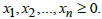
2.2. General Form of Linear Programming
- The general form of a linear programming problem is expressed in the form:Maximise (Minimise)
 (objective function)Subject to
 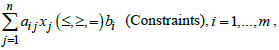 and
and  (Non-Negativity Constraints)
  Where
Where is the decision variable,
  is the net unit contribution of the decision variable
  to the value of the objective function,
  denotes the total availability of the
  resources and
  stand for the amount of resources, say
  consumed in making one unit of project
  . The general form can also be expressed in the form:Maximise (Minimise)
 Subject to the constraints
  | (1) |
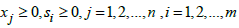
2.3. Standard Form of Linear Programming
- The main characteristics of linear programming in standard form are i. All variables are non-negative.ii. The right-hand side of each constraint is non-negative.iii. All constraints are expressed as equations using slack and surplus variable
 .Therefore, equation (1) can be expressed in standard form as: Maximise
 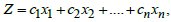 Subject to
 | (2) |
2.4. Duality
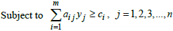
- According to [16], duality, or the duality principle, emphasizes that optimization problems can be approached from two angles: the primal problem or the dual problem. The given original problem is the primal programme. This programme can be written by transposing the rows and columns of the original problem which results in the dual programme. When the primal problem involves minimizing, the dual involves maximizing (and vice versa). Any feasible solution to the primal (minimization) problem is at least equal to any feasible solution to the dual (maximization) problem. One important aspect of the duality of a linear programming problem is that it checks the accuracy of the primal solution. Suppose the primal is expressed as:Maximise
 Subject to the constraints
 | (3) |
 Then, the dual problem for equation (3) is expressed as:Minimise
 | (4) |
 and
and  is the dual variable which represent the shadow price for the primal constraints.Theorem 2.1The value of the objective function
  for any feasible solution of the primal is
  the value of the objective function
  for any feasible solution of the dual.ProofMultiply the first inequality in equation (3) by
  , the second inequality by
  etc. and add them all. This results in:
 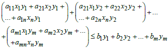 | (5) |
 , the second inequality by
  etc. and add them all. This results in:
  | (6) |
 | (7) |
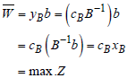
 .Theorem 2.2 (Fundamental theorem of duality)If both the primal and the dual problems have feasible solutions then both have optimal solutions and max.
  = min.
  .ProofExpress the dual primal problem in symmetric form as:
 | (8) |
 | (9) |
 and the corresponding optimal value of the primal objective function be
  | (10) |
 | (11) |
 | (12) |
 and
and  ,
, Which will also be true for extreme optimal and dual values
 | (13) |
 cannot be less than
  Therefore
2.5. Basic Terminologies
2.5.1. Loan
- A loan refers to the transfer of money, property, or other material goods from one party to another with the agreement that the recipient, or borrower, will repay the amount along with an additional sum known as interest [17]. The borrower incurs a debt and is obligated to pay interest for the use of the money.
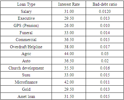
2.5.2. Interest Rate
- The interest rate is the percentage of the principal amount that a lender charges as interest on the money borrowed. It is a critical factor in determining the cost of borrowing and the return on investment. In the context of linear programming, the interest rate can be a parameter in financial models, affecting the optimization of investment portfolios, loan repayment strategies, or managing interest rate risk [18].
2.5.3. Bad-Debt Ratio
- The bad-debt ratio is a financial metric that measures the percentage of money a company has to write off as a bad debt expense compared to its net sales. It indicates what percentage of sales profit a company loses to unpaid invoices [19].
2.5.4. Shadow Price
- In linear programming, shadow prices represent the change in the optimal value of the objective function per unit change in the constraint. In instances where resources are scare, the shadow price indicates how much the objective function value would increase or decrease if there was a marginal increase in the availability of that resource by one unit, assuming all other constraints remain unchanged. They provide insights into the value of additional resources or changes in constraints, helping to optimize production or allocation strategies.
3. Data Analysis and Results
3.1. Study Data
- The data used in this study are secondary data obtained from a financial institution. This dataset includes various types of loans granted by the financial institution, their corresponding interest rates, and the bad-debt ratio. The data for the study is presented in Table 1.
|
3.2. Model Assumptions
- The following are the various assumptions considered by the financial institution when allocating funds for loans:1. The bad-debt ratio should not exceed 3% of all loans.2. A maximum amount of 189,729,929.00 has been allocated for loan during the 2023 financial year.3. The total amount allocated for the various types of loans should not exceed 45% of the total amount of funds allocated for loans within the 2023 calendar year.
3.3. Formulation of the Linear Programming Model (LPM)
- To formulate the loan model using linear programming, the objective function is deduced subject to some linear constraints.
3.3.1. Assigning Decision Variables
- In this study, the following variables are utilized to represent the key decision-making factors under consideration;Let
 = Amount to be invested in Salary loans
  = Amount to be invested in Executive loans
 = Amount to be invested in Ghana Police Service loan
 = Amount to be invested in Funeral loans
 = Amount to be invested in Commercial loans
 = Amount to be invested in Overdraft loans
 = Amount to be invested in Agric loans
 = Amount to be invested in Auto loans
 Amount to be invested in Church development loans
 = Amount to be invested in Susu loans
 = Amount to be invested in Microfinance loans
 = Amount to be invested in Gold loans
 = Amount to be invested in Asset loans
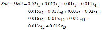
3.3.2. Formulation of the Objective Function
- To formulate the objective function, linear equations related to the interest and debt ratio are formulated as part of the linear equation. Therefore,
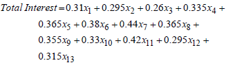 | (14) |
 | (15) |
 | (16) |
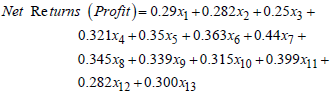 | (17) |
 | (18) |
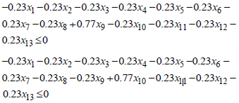
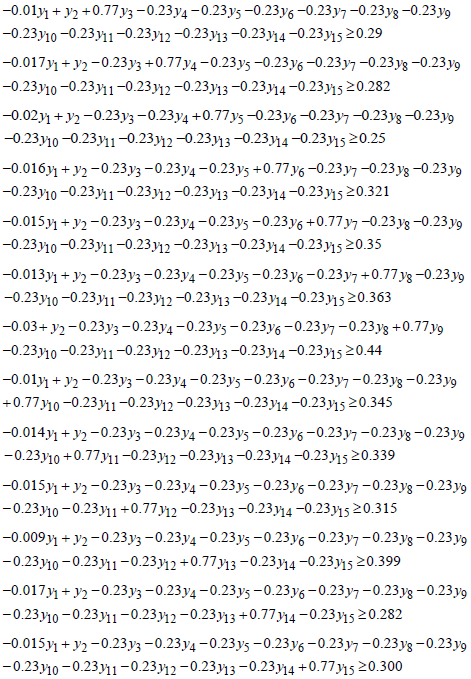
3.3.3. Formulation of the Constraints
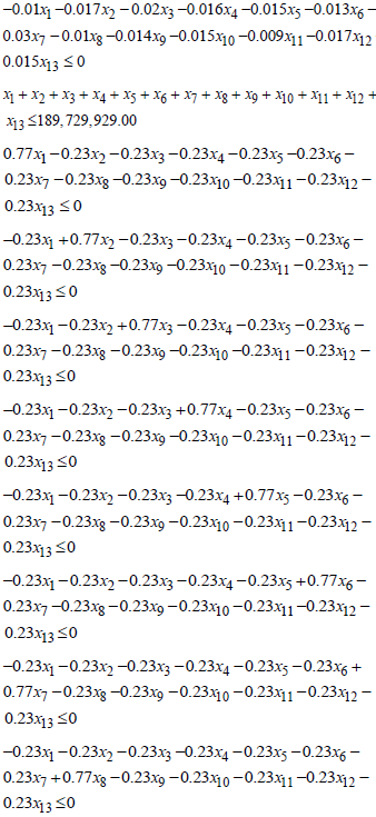
- From the model assumptions and the policies of the financial institution, the constraints relating to the objective function are deduced as follows:i. The bad-debt ratio should not be more than 3% of all loans granted implies that;
 ii. The amount allocated for loans in the 2023 financial year should not exceed GH
 189 729 929.00. This implies that,
  iii. The amount invested in each of the loan types should not exceed 23% of the total amount allocated for loans. This also implies that; For
  , if
, if 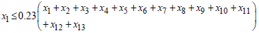 Then,
Then,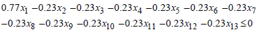 For
For  , if
, if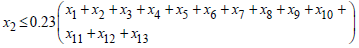 Then,
Then,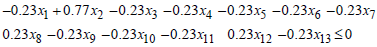 For
For  , if
, if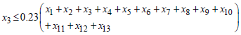 Then,
Then,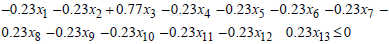 For
For  , if
, if  Then,
Then, For
For  , if
, if  Then,
Then,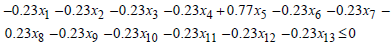 For
For  , if
, if 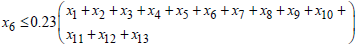 Then,
Then, For
For  , if
, if  Then,
Then, 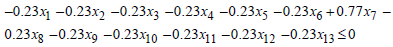 For
For  , if
, if 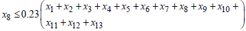 Then
Then  For
For  , if,
, if,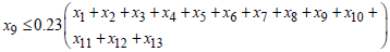 Then
Then For
For  , if
, if 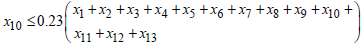 Then,
Then, 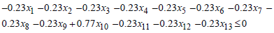 For
For  , if
, if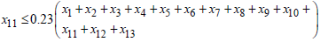 Then,
Then,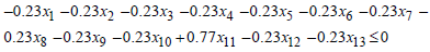 For
For  , if
, if 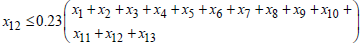 Then,
Then, 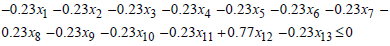 For
For  , if
, if  Then,
Then,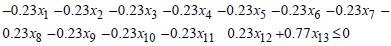 Thus, the formulated linear programming model aimed at maximizing loan returns for the financial institution can be expressed as follows:Maximise
  | (19) |
 and the non-negativity constraints,
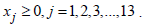
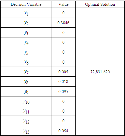
3.4. Optimal Solution
- Due to the number of constraints and decision variables involved, the QM solver for window software was used to solve the linear programming based on the simplex method. The optimal solution of the proposed model is indicated in Table 2.
|
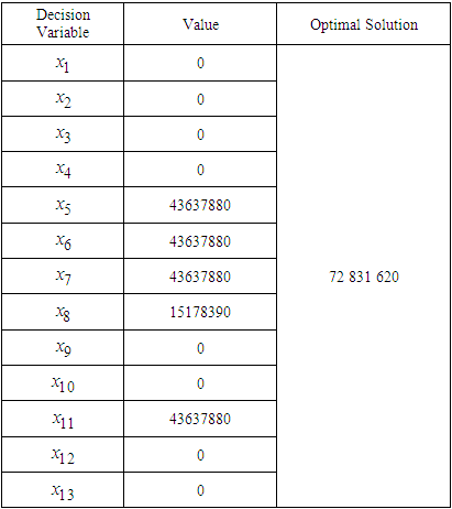
 43 637 880.00 to Commercial loans, GH
 43 637 880.00 to Overdraft/Helpline loans, GH
 43 637 880.00 to Agric loans, GH
 15 178 390.00 to Auto Loans, and GH
 43 637 880.00 to Microfinance loans.This allocation results in an optimal profit of GH
 72 831 620.00.It's worth noting that while the bank still generates profit from its initial allocations, to maximize profitability, the bank should refrain from investing in Salary loans, Executive loans, Ghana Police Service loans, Funeral loans, Church development loans, Susu loans, Gold loans, and Asset loans.
3.5. Post-Optimality Analysis
- This section presents the Sensitivity Analysis of the study. In this analysis, certain coefficients of the decision variables will be varied to assess their impact on the optimal solution.
3.5.1. Sensitivity Analysis
- According to [20], sensitivity analysis is a financial modelling technique that helps to determine how changes in one or more input variables affect the output of a model. It is a way to predict the outcome of a decision given a certain range of variables. Therefore, the profit coefficient for the objective function equation (20) is systematically adjusted to assess its influence on the optimal solution. This adjustment is detailed in Table 3.
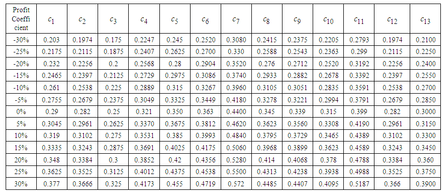 | Table 3. Change in Profit Coefficient |
|

 50,982,130.00. Similarly, a 25% reduction led to a decrease of GH
 54,612,800.00, while a 20% reduction resulted in a decrease of GH
 58,370,020.00. A 15% reduction caused a decrease of GH
 62,018,160.00, and a 10% reduction resulted in a decrease of GH
 65,666,280.00. A 5% reduction led to a decrease of GH
 69,314,410.00. Maintaining the profit coefficient unchanged yielded an optimal outcome of GH
 72,831,620.00.Conversely, when there was a 5% increase in the profit coefficient, the optimal outcome rose to GH
 76,610,660.00. A 10% increase led to an increase of GH
 80,258,780.00, while a 15% increase resulted in an increase of GH
 83,906,150.00. A 20% increase caused an increase of GH
 87,555,040.00, and a 25% increase resulted in an increase of GH
 91,203,170.00. Finally, a 30% increase in the profit coefficient led to an increase of GH
 94,851,300.00. These findings illustrate a consistent pattern: an increase in the profit coefficient corresponds to an increase in the optimal value, while a decrease in the profit coefficient corresponds to a decrease in the optimal value.
 3.6. Dual of the Linear Programming Model
- Duality provides alternative viewpoints to approach and analyze linear programming problems. It allows the examination of the problem from different angles, often leading to new insights and validating the solutions. Therefore, this section investigates the validity of the optimal solution obtained in Table 2. The dual problem of the linear programming model in equation (20) is formulated, and its optimal solution is also determined. Hence, The Duality Form of the linear programming is written as:Minimise
 | (20) |
 Where
Where 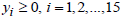 .Table 5 indicates the duality form of the decision variables, their respective values and the optimal solution using QM Solver software.
|
 +
+  +
+  +
+  +
+  +
+ +
+  +
+  +
+ +
+ +
+  +
+  +
+  and the dual problem (
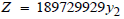 ) are the same (GH
 72,831,620). This validates the solution of the linear programming problem, as stated in theorem 2.2 The decision variables of the dual problem represent the shadow prices. For instance,
  = 0.3846 implies that if the primal model is increased or decreased by GH
 1, the optimal solution (profit returns) will also be increased or decreased by GH
 0.3846. Similarly,
  , implies that if the primal model is increased or decreased by GH
 1, the optimal solution (optimal investment) return will also be increased or decreased by GH
 0.005. This relationship continues with
  and
and  , where each represents the impact of changes in the primal model on the optimal investment return.
4. Discussion
- The developed loan model holds significant potential to assist the financial institution by serving as a guiding tool when making loan decisions, ultimately optimizing profits since the It's worth recalling from the sensitivity analysis conducted on the developed model that, as profit coefficients decrease, optimal profits decrease, and conversely, when profit coefficients increase, optimal profits rise. This means that there is a positive relationship between the profit returns and the change in the profit coefficient as indicated in Table.Additionally, it should be noted that both the Primal Model and the Dual Model yield identical optimal solutions, in accordance with the Strong Duality Theorem discussed in Chapter Three. This provides further validation of the robust formulation of both models.Lastly, the results of the duality analysis offer an added advantage, as one can determine the impact of resource availability changes on the optimal solution or profit returns without the need to run the developed loans model as indicated in Table 5.
5. Conclusions
- A well-constructed linear programming model has been created to maximize the return on loan investments at the financial institution, as depicted in equation (20). The optimal solution reveals that the bank stands to achieve a maximum profit of 72,831,620 Ghana Cedis.The sensitivity analysis conducted to assess the impact of profit coefficient variations clearly demonstrates a direct correlation between the profit coefficient and the resulting optimal solution. These findings are detailed in Table 4.The duality analysis conducted on the developed model reveals that the dual model shares the same optimal solution as the primal model, which amounts to 72,831,620 Ghana Cedis. This validates the accuracy of the model formulation and also affirms the duality theorem.
ACKNOWLEDGEMENTS
- The authors of this article gratefully acknowledge the management of the financial institution in the Prestea-Huni-Valley District for generously providing us with the secondary data essential for this study.