RRK Sharma1, Shivam Saini1, Omprakash K. Gupta2, Vinay Singh3
1Dept of IME IIT Kanpur, 208016, India
2University of Houston – Downtown Houston, TX, USA
3AB-IIIT Gwalior, India
Correspondence to: RRK Sharma, Dept of IME IIT Kanpur, 208016, India.
| Email: |  |
Copyright © 2023 The Author(s). Published by Scientific & Academic Publishing.
This work is licensed under the Creative Commons Attribution International License (CC BY).
http://creativecommons.org/licenses/by/4.0/

Abstract
Plant layout problems are well researched problems (see Singh and Sharma [10]) for references. SPLPs (simple plant layout problem) are single period problems where one allots facilities to slots so that sum total of material handling cost is minimized; whereas DPLPs (dynamic plant layout problem) are multi-period problems. In DPLP the flows between facilities or machines change as old products are weeded out and newer ones are added. This necessitates that facilities be relocated to different slots so that we have minimized the sum total of relocation cost and the material handling cost. These problems are known to be NP-Hard. Multi-Floor (MF) layout problems are more complex. Here we give four new model on MF-SPLP. Novel formulations and its new linearization(s) are given. We also give details of computational investigation carried out by us.
Keywords:
Simple plant layout problem (SPLP), Multi floor (MF) plant layout problems, MF-SPLP
Cite this paper: RRK Sharma, Shivam Saini, Omprakash K. Gupta, Vinay Singh, New Model on Multi Floor Simple Plant Layout Problems (MF-SPLP), American Journal of Operational Research, Vol. 13 No. 1, 2023, pp. 1-7. doi: 10.5923/j.ajor.20231301.01.
1. Introduction
The simple plant layout problem (SPLP or the quadratic assignment problem QAP) is posed as follows. There are N slots where N facilities are to be located. Distance between slot ‘j’ and ‘l’ is known and denoted by D(j,l). The material flow between machines (facilities) are known in advance (it is determine by product mix of the company and technological requirements of sequence in which different operations are performed on different jobs). We seek to minimize the material handling cost of the total shop when all machines are considered. It results in quadratic objective function involving binary variables s.t. linear constraints. It is a single period problem. When material flow between machines changes (due to change of product mix of the company in different time periods) a multi-period problem results when machines are dismantled from one location and placed in other slot. This multi-period problem is referred to as dynamic plant layout problem (DPLP). Below we give formulation of QAP. Problem QAP or SPLP– 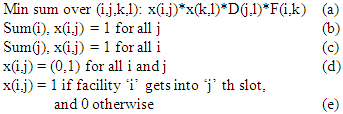 D(j,l) is the distance between ‘j’ th and ‘l’ th slot and F(i,k) is flow between facility ‘i’ and ‘k’. Now we give here classic formulation of DPLP or the dynamic multi-floor plant layout problem. Problem DPLP–
 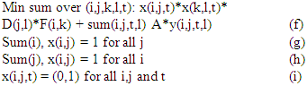 also we have y(i,j,t,l) as binary variable that is 1 if ‘i’ th facility in slot ‘j’ in period ‘t’ goes to slot ‘l’ in period ‘t+1’ and 0 otherwise. This is achieved by following equations.
  it s easy to see that this requires that y(i,j,t,l) be real and greater than or equal to 0; and not binary (see Singh and Sharma (2008)) (k)
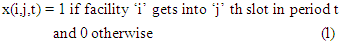 D(j,l) is the distance between ‘j’ th and ‘l’ th slot and F(i,k) is flow between facility ‘i’ and ‘k’. It is well known that problem SPLP is NP-Hard and computationally intractable. Hence heuristics are popularly used to solve QAP. These are Genetic Algorithms, Tabu Search, Simulated Annealing etc. For a detailed exposition refer to [13]. This makes (use of heuristics and meta heuristics) sense as SPLPs and DPLPs are intractable problems (they are NP-Hard) and optimization based exact algorithms will take exponential amount of CPU time as problem size increases. Researchers also have tried to linearize the objective function by adding more real and/or binary variables. A summary formulations of different formulations for SPLP are given in Loiola et al. [6] and various linearizations of SPLP are given in [14]. And a table of comparison is reproduced here.
 Table 1. Comparison of Sizes of Different Formulations and Linearization of QAP
 |
| |
|
In this paper we give new linearization(s) of MF-SPLP, MF-DPLP and ‘sequence’ dependent MF-DPLP. MF-SPLP is a single period problem; whereas MF-DPLP is a multi-period problem. In ‘sequence’ dependent MF-DPLP the relocation cost depends not only on where it is relocated but also depends on from where it is lifted. Here the new linearization has much less number of binary variables. Reader is referred to [9], [11] and [12] for latest details. Since both SPLP and DPLP are computationally intractable exact methods are not advised. Literature is flooded with the application of Genetic Algorithm, Simulated Annealing and Tabu Search methods for solving SPLP and DPLP (see Singh and Sharma [13]).
2. A New Linearization of Multi Floor Simple Plant Layout Problem (SPLP)
Here we describe the multi-floor problem considered in this paper in detail. In normal SPLP all the slots (where facilities can go) are on the ground floor. There are multi-bay SPLPs where slots are arranged in multiple bays and facilities are located there. There is premium on ground space and hence sky rise buildings are more common now a days. So we have a multistoried building that has ‘J’ floors and each floor has exactly ‘K’ slots. So there are a total of J*K slots where exactly J*K facilities are to be located such that sum total of material handling cost is minimized. This problem can be solved by posing it as problem QAP (((a) to (e)) above. Here if there are N slots and N floors, the associated QAP has N4 binary variables. We give here a new formulation of MF-SPLP that has only N2 binary variables and has other advantages. We give the formulation below. Constants of the Problem: i index for facility; j index for floor and k index for slot. D(j1,k1, j2,k2) = distance between slot k1 ant floor j1 and slot k2 at floor j2. F(i1,i2) = flow between facility i1 and i2. Decision Variables: X(i,j) = 1 if facility ‘i’ is on floor ‘j’ and 0 otherwise.Y(i,k) = 1 if facility ‘i’ is in slot ‘k’ and 0 otherwise. Problem Formulation: P1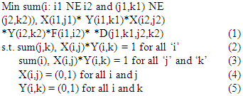 Linearization: we introduce variables Z(i1,j1,k1,i2,j2,k2) = (binary variables = (0,1))X(i1,j1)*Y(i1,k1)*X(i2,j2)*Y(i2,k2) and then we have the following:
  s.t. (2) & (3), and
 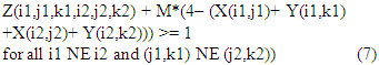 It can be easily seen that (as in [16]), Z(i1,j1,k1,i2,j2,k2) need not be binary but need to be positive real variables (Z(i1,j1,k1,i2,j2,k2) >= 0). We hope that this is new linearization of Multi-Floor SPLP. It has only N*(S+F) binary variables (where N is number of facilities, S is max no of slots and F is max number of floors). Objective function can be posed as:
  Other formulation possible is also given here (probably given in literature): X(i1,j1,k1) = 1 if facility i1 is located on floor j1 and slot k1 (on floor j1 only); and 0 otherwise. Other constant definitions are same and then multi-floor SPLP is: Problem Formulation P2: Min (6)
 Linearization: we introduce variables Z(i1,j1,k1,i2,j2,k2)= (binary variables = (0,1))X(i1,j1,k1)*X(i2,j2,k2) and then we have the following: Min sum(i1 NE i2 and (j1,k1) NE (j2,k2)), Z(i1,j1,k1,i2, j2,k2)*F(i1,i2)*D(j1,k1, j2,k2)s.t. (9), (10) and (11) &
 It can be easily seen that (as in [16]), Z(i1,j1,k1,i2,j2,k2) need not be binary but need to be positive real variables (Z(i1,j1,k1,i2,j2,k2) >= 0). Here we have N2 binary variables (where N is number of facilities).We offer one more novelty in formulation P2. We introduce binary variables X1(i1,j1) to be equal to ‘1’ if facility ‘i1’ goes to floor ‘j1’ and zero otherwise; and Y1(i1,k1) to be equal to 1 if facility i1 goes to slot k1 and zero otherwise. And we introduce additional constraints.
  Now with this it is easy to see that X(i1,j1,k1) need not be binary but can be greater than zero and real. This so because, if X(i1,j1,k1) is to be greater than ‘0’, then it will have to be at ‘1’ due to constraints (13) and (14) & (15). If any of the X1(i1,j1) or Y1(i1,k1) is equal to ‘0’, then constraint (13) and (14) will force it (X(i1,j1,k1)) to be equal to ‘0’.It is easy to see that (7) can be used in place of (12).Now we are in a position to give a new formulation of MF-SPLP (posed as problem P3). Problem P3: (6) s.t. (7), (9), (10), (13), (14), (15) and (16)
 Thus we have reduced number of binary variables in formulation P3, which is expected to make it more efficient. Computational investigation is underway and results will be reported soon. Now we give yet another formulation of MF-SPLP (posed as problem P4).Problem P4: (6) s.t. (9), (10), (13), (14), (15), (16), (12) and (17)
Table 2. Comparing Four Formulations of MF-SPLP
 |
| |
|
As we go ahead with this a paper, a yet new formulation of MF-SPLP is given below as problem P5. Problem P5: Min (8); s.t. (9), (10), (16), (13), (14), (15) and (4), (5). It has quadratic objective function in real variables with linear constraints. It has N2 real variables and has N*(S+F) binary variables. It will be worthwhile comparing efficacy of above two formulations P1, P2, P3, P4 and P5; and also respective linearization that are a measure of lower bound. It can be seen that model P1 has non-linear constraints, but model P3 has perfectly linear constraints (with quadratic objective function in real variables) with lesser number of binary variables which is likely to make it more efficient than P1 or P2. Similarly, P4 has more real variables than P3, but has linear objective function in real variables. Here we give results of empirical investigation undertaken to determine the efficacy of these models.
3. Discussion
In this paper we give a new formulation (P3) of multi floor SPLP that has least number of binary variables and is a perfectly a linear model but has quadratic objective function in real variables. We also give a new problem formulation that has additional [N*S*F)]2 real variables but has linear objective function in real variables. This is a useful contribution we make. Similar contribution are possible for MF-DPLP (multi-floor dynamic plant layout problem).
4. Computational Results
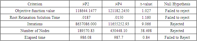
A total of 30 problems of size 3*3, 4*4, and 5*5 were solved (models P2, P3 and P4 were solved on AMD Ryzen 5 4500U with Radeon Graphics 2.38 GHz.), and the data for these problems was randomly generated. 3*3 Problem: Here we considered 3 floor and each floor has 3 different slots in which total 9 facilities can be located. Then we utilized GAMS programs for different models, which were used to implement the solution technique in a step-by-step manner. Results we get after running GAMS program are reported here. As P1 turns out to be infeasible so we only reported results of P2, P3, and P4.Table 3. Comparison Table between P2 and P3: 3 by 3 Problems
 |
| |
|
Model P2 is better than P3 which is supported by statistical test as Model P2 shows significant improvements in terms of iterations, number of nodes and root mean time, with lower values compared to P3.Table 4. Comparison Table between P3 and P4: 3 by 3 Problems
 |
| |
|
P3 is a better option than P4 for situations where number of iterations and no of nodes processed is important; as it can be inferred that there is no significant change in objective function value for both models P3 and P4. Table 5. Comparison Table between P2 and P4: 3 by 3 Problems
 |
| |
|
It can be concluded that model P2 and P4 are equally good as there is no statistical difference between both in case of objective function; but P2 is superior to P4 in terms of no of nodes processed and no of iterations. Thus P2 is best among P2, P3 and P4 for 3 X 3 sized problems. 4*4 Problem: Here we considered 4 floor and each floor has 4 different slots in which total 16 facilities can be located. Then we utilized GAMS programs for different models, which were used to implement the solution technique in a step-by-step manner. Results we get after running GAMS program are reported here. As P1 turns out to be infeasible so we only reported results of P2, P3, and P4.Table 6. Comparison Table between P2 and P3: 4 by 4 Problems
 |
| |
|
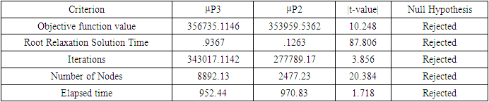
P2 outperforms model P3, as it shows significant improvements in terms of objective function, root mean time, iteration, and number of nodes with lower values compared to P3. Table 7. Comparison Table between P3 and P4: 4 by 4 Problems
 |
| |
|
Table 8. Comparison Table between P2 and P4: 4 by 4 Problems
 |
| |
|
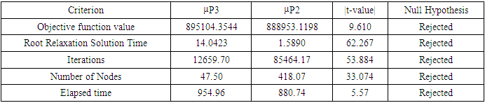
It can be concluded that model P3 and model P4 are equally good, as P3 shows significant improvements in terms no of iterations iteration, and number of nodes with lower values compared to P4 (it takes significantly less CPU time (with elapsed time used as proxy)). But P4 shows significant improvement in the value of objective function. It can be concluded that model that no models is clearly superior, as P2 shows significant improvements in terms of iteration number and number of nodes with lower values compared to P4. But P4 shows significant improvement in the value of objective function. So P3 and P4 are good models for 4 X 4 sized problems. 5*5 Problem: Here we considered 5 floor and each floor has 5 different slots in which total 25 facilities can be located. Then we utilized GAMS programs for different models, which were used to implement the solution technique in a step-by-step manner. Results we get after running GAMS program are reported here. As P1 turns out to be infeasible so we only reported results of P2, P3, and P4.Table 9. Comparison Table between P2 and P3: 5 by 5 Problems
 |
| |
|
Model P2 outperforms model P3, as it shows significant improvement in terms of objective function with lower values compared to P3. But P3 takes significantly less no of iterations and no of nodes processed. Table 10
 |
| |
|
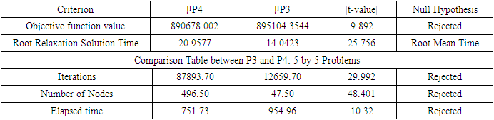
It can be concluded that no model is clearly superior, P3 shows significant improvements in terms of iteration and number of nodes with lower values compared to P4. But P4 shows significant improvement in the value of objective function.Table 11. Comparison Table between P2 and P4: 5 by 5 Problems
 |
| |
|
P2 outperforms model P4, as it shows significant improvement in terms of elapsed time, iterations and number of nodes with lower value compared to P4. Also P2 shows significant improvement in the value of objective function. A point in favor of P4 is that for 5 X 5 problems, it takes least CPU time (with elapsed time used as proxy). P2 is better among all for 5 X 5 problem. Based on above results and inferences we can conclude that model P2 turns out to be best model among P1, P2, P3 and P4 for MF-SPLP for 5 X 5 problems. P3 and P4 are good models for problems of size 4 X 4. For 3 X 3 sized problem models P2, P3 and P4 are as good; none clearly superior. All the above problem instances were solved again (The computation was done on the machine specification HP made Intel core(TM) i5 CPU @ 3.20 GHz, Installed Memory 4.00 GB, 32-Bit Windows 7. OS) by model P5 in GAMS and for 3 X 3 and 4 X 4 sized problems. Results are given below. 3 X 3 Sized Problems Solved by Model P5
 |
| |
|
4 X 4 Sized Problems Solved by Model P5
 |
| |
|
3 X 3 problems have 54 binary variables whereas 4 X 4 problems have 128 binary variables. P5 is very fast (around 300 times faster) and gives good solutions. We can solve models P2, P3 or P4 by using the advanced starts given by model P5 in very short (elapsed) time. Problems 5 X 5 had 250 binary variables. These problems were solved and returned no solution (GAMS called it as infeasible) except for one problem (problem no 8 which had a solution far away from the solutions given by either P2, P3 or P4). It so turns out that problem of size 3 X 3 or 4 X 4 be solved by first by model P5 and then the solution so returned can be fed to other models (P2, P3 or P4) to reach to a better solution. This is because model P5 takes very little elapsed time to return a good solution. Problems of size 5 X 5 or above can be fed directly to model P2, P3 or P4. This is the conclusion that follows from this paper. The above results can be viewed in light of the fact that SPLP with number of facilities equal to 27 is NOT solvable optimally by commercially available software [10].
Conflict of Interest
All authors listed above (for this paper) received NO research grants from any Company for conducting this research and preparing this paper. All Authors declare that they (he/she) have no conflict of interest.
Ethical Approval
This article (with above title and authors) does not contain any studies with animals performed by any of the authors. This article (with above title and authors) does not contain any studies with human participants or animals performed by any of the authors.
References
| [1] | Assad, A. and Xu, W., “On lower bounds for a class of quadratic 0-1 programs”, Operations Research Letters, V 4(4), 1985, p. 175-180. |
| [2] | Christofides, N. et. al., “Contributions to quadratic assignment problem”, European J of Operational Research, V 18(4), 1980, p. 243-247. |
| [3] | Frieze, AM and Yadegar, J., “On the quadratic assignment problem”, Discrete Applied Mathematics, V5, 1983, p. 8998. |
| [4] | Kauffman L. and Broeckx, F., “An algorithm for quadratic assignment problem using Bender’s decomposition”, European J of Operational Research, V2, 1978, p. 204-211. |
| [5] | Lawler LE, “The quadratic assignment problem”, Management Science, 1962, 586-599. |
| [6] | EM Loiola et. al, “A review of QAP”, European Journal of Operational Research 176 (2007), p. 657–690. |
| [7] | Padberg, W. and Rijal, P., “Location, Scheduling, Design and Integer Programming”, Kluwer Academic Publishers, Boston, 1996. |
| [8] | R Shriniwas Sharma, RRK Sharma, Vinay Singh and SP Singh, “A lagrangian based procedure for solving simple plant layout problem”, Journal of Academy of Business and Economics, V12(1), 2012; pp. 161-166. |
| [9] | RRK Sharma, “Working Paper Series: Lecture Notes in Management Science: Vol 6”, (It has 048 articles are written so far: All Authored by Prof. RRK Sharma); ISBN: 978-93-91355-65-4; May 2022. |
| [10] | Singh, S.P., “Solving the Static and Dynamic Plant Layout Problems: Developing a few GA and SA based heuristics”, PhD Thesis at the Department of Industrial and Management Engineering, Indian Institute of Technology, Kanpur 208016 (completed 2007). |
| [11] | Singh, S.P. and Sharma R.R.K., “A review of different approaches to the facility layout problem”, International Journal of Advanced Manufacturing Technology, 2006, V30, 425-433. |
| [12] | Singh, S.P. and Sharma R.R.K., “Two-level modified simulated annealing based approach for solving facility layout problem”, International Journal of Production Research; V 46(13), July 2008, pp. 3563 – 3582. |
| [13] | Singh, S.P. and Sharma, R.R.K., “Genetic algorithm based heuristic for the dynamic facility layout problem”, European Journal of Management, V8(1), 2008, pp. 128-134. |
| [14] | Sharma, R.R.K. and Singh, S.P., “A review of various linearization of the QAP: A comparative study for assessing relative computational effort”, Review of Business Research, V8(1), 2007, pp. 185-190. |

 Abstract
 Reference
 Full-Text PDF
 Full-text HTML