F. O. Ohanuba1, 2, P. N. Ezra2, N. M. Eze2
1School of Mathematical Sciences, Universiti Sains Malaysia, Penang, Malaysia
2Department of Statistics, University of Nigeeria, Nsukka
Correspondence to: F. O. Ohanuba, School of Mathematical Sciences, Universiti Sains Malaysia, Penang, Malaysia.
| Email: |  |
Copyright © 2020 The Author(s). Published by Scientific & Academic Publishing.
This work is licensed under the Creative Commons Attribution International License (CC BY).
http://creativecommons.org/licenses/by/4.0/

Abstract
This study centers on effective financial management via suitable decision planning to invest in a competing stock portfolio and sets to clearly describe the procedure of Markowitz’s Portfolio Theory in-stock selection and apply a table-like method in solving the stock allocation portfolio problem in DP. There has been problem of how to choose a stockportfolio to invest a revenue for optimal return among investors, in financial market. Most financial analyst on the other hand mislead investors by choosing the wrong stocks for investment and using the traditional method that will only give minimal optimum return. In order to solve these problems, our study extended the work of Yan and Bai, and solved company's financial problem using a simplified tabular-method: we described how the Modern Portfolio Theory (MPT) is used in stock selection. The traditional procedure of solving the financial problem is complicated and cannot trace the path to the global maximum return. Moreover, the introduced table-like method deals with portfolio problem with minimum transaction lots and also check the limit outside which the calculation, including the steps, are irrelevant. Besides, the adopted technique makes the computation easy and precise. The metric unit (Ringgit Malaysia) is used in this work to suit the researcher's address. This study also shows a network representation of the nodes and connection between nodes. The network displays how each stage connects to the other by connectors. The network presentation makes the procedure precise and better explained. Case one in the application shows that tabular method gives an optimal result as shown in the work of Yan and Bai. The impact of the study is shown in case two where a global optimum return (RM3, 400,000) is achieved in table 9 compare to RM3, 300,000 in table 5 where the control variable was not used. The path that lead to global optimum can be traced using the network presentation.
Keywords:
Dynamic programming, Portfolio, Stocks, The global maximum, Reverse algorithm
Cite this paper: F. O. Ohanuba, P. N. Ezra, N. M. Eze, On the Financial Optimization in Dynamic Programming via Tabular Method, American Journal of Operational Research, Vol. 10 No. 2, 2020, pp. 30-38. doi: 10.5923/j.ajor.20201002.02.
1. Introduction
Revenue management in a financial stock portfolio has caused a great shock to the global economy. It has led to the collapse of many global stock markets due to lack of proper information on business strategy. The word "programming" in "dynamic programming" is similar for optimization. It is the same as “planning” or a “tabular method”. Dynamic programming, DP involves a selection of optimal decision rules that optimizes a specific performance criterion. The 3 main problems of S&P 500 index, which are single stock concentration, sector risk and style risk, are being taking care of in this study. The tabular method introduced in this study gives a robust result and explains in detail the procedures for solving financial problem, from the stage one to the last step (stage four). Having identified a gap in DPP (dynamic programming problem), we propose a table technique method. According to Hamdy, DP can determine the optimum solution to an n-variable problem by decomposing it into n stages consisting of single variable sub-problems [1]. Hamdy, in his work, stated that the nature of the stage differs, depending on the optimisation problem. DP does not provide computational details for optimisation of each stage, and this study filled the gap in the tabular method introduced. On the course of optimisation in investment, [2] developed a theory on portfolio selection and fund allocation strategy, especially among a variety of stocks so that investors make maximum benefit from the portfolio. [3] Solved an existing financial problem of a company using the general dynamic programming model developed by Richard Bellman and their method does not apply the table-like technique for better understanding. They converted the financial stock portfolio problem to a dynamic programming problem using some dynamic terminologies. We incorporated both the principle of optimality, which follows a recursive procedure to solve a company’s financial problem. [4]. In their paper presented the result of a case study of the decision-making processes of investment managers in developing economies. The article stated that natural setting contributes to the importance of the security of investment. Also, adequate networks, consistency of returns, management competency, stable environment, legal and regulatory controls are core investment decision making concepts. Modern Portfolio Theory (MPT) proffers solution on how to allocate funds rationally among a variety of stocks. Markowitz's work is the key to making the best returns with the least amount of risk on portfolios with different asset risk. MPT was used to select a portfolio-asset with minimum risk to invest. This selection helps investors to minimize risk in the course of portfolio selection. The procedure of MPT is by assigning the weight to the portfolio and comparison of covariance between assets with minimum weight (lowest variance). This study centres on effective financial management via suitable decision planning to invest in a competing stock portfolio and sets to achieve these objectives:(i) To clearly describe the procedure of Markowitz’s Portfolio Theory in-stock selection.(ii) To apply a table-like method in solving the stock allocation portfolio problem in DP.This research is the first to apply a table-like technique in solving the financial problem of a company; this is a motivation in this study. Besides, many investors usually do not know how to choose (select) from varieties of stocks. The procedure of this method is simplified and concise and observed the recursive process of the principle of optimality. Bellman’s dynamic programming model was modified to suit our approach. [3] Solved a company's financial problem with a different technique, but their method is more complex and does not show the detailed procedures of optimization of the DPP. Yan and Bai in their solution to the company’s problem, did not show optimal value at each stage, which our approach does. We introduced a variable of control into the model, and we called it, the state control variable  .The function of the state control variable
  is to check the limit outside which the calculation might be irrelevant. The introduction of the variable also helped the researchers to obtain a global maximum in the final return. Most of the kinds of literature reviewed have not considered the table-like approach. The beauty of this approach is that all the procedures follow a simple descriptive form, which can easily be understood by investors. [5] In their paper focused on American option pricing and portfolio optimisation problems when the underlying state space is high-dimensional. Haugh handled the issue of dimensionality using approximate dynamic programming (ADP) methods. Other literatures we consulted in the course of this study and for further research are; [6-14].
2. Material and Methodology
The methodology applied in this study is called a table-like method and the investment problem solved is shown in table 1: where a company/investor buys from four stocks. The problem also shows the relationship between return (unit: RM10, 000 per unit) and investment (unit: RM10, 000 per unit) of each stock. The investment is measured in unit and the total amount the company invested is 6units = RM60,000 and the basic principles of choosing the four stocks is explained in MPT: The recursive solution to the problem is explained in the basic principle of dynamic programming. It follows iterative and recursive procedures in its computation. The introduction of the control variable modified the model of Bellman and introduced a control variable to suite our method, as shown in the following model: Where S = Total investment, n = Item number of the portfolio,
  = Decision variable, investment assigned to item K,
  = Stage objective function, return of
  = State variables, investment of item k to item n,
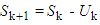 is the state transition equation,
  Maximize return of
  is the control variable introduced and which tentatively lie between 0 to 10. The range is arbitrarily chosen for this study, and the study is limited to stage four. If we let
  and
and  , we can recover the original model of Bellman. The procedure adopted for this work is presented in equations 2.1 to 2.6.Let
  be a vector (called state variable) containing a variable to be selected at stage j, j represents the various stages, and for any particular problem, n is the last stage. At j = 2, for instance, implies the second stage of the problem.
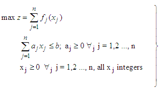 | (1) |
The computational method which yields an optimal solution to 2.1, and indeed yields all alternative optimal solution is unique  , and
, and  in 2.1 are assumed to be integers. This is not really any restriction; the restriction only limits the selection of physical dimensions used to measure
  and
and  . Maximization of z can be carried out in any way we like, provided that the method makes it possible to examine every set of feasible
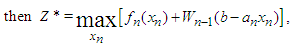
  if it is desirable to do so. That is when the recursive principle is observed. Denote z* the absolute maximum of z in 2.1. Then
 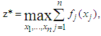 | (2) |
Where the maximization is carried out for non-negative integers  satisfying
 | (3) |
We proceed by selecting a value of  and holding
  fixed, maximize z over the remaining variables, that is, over
  . The values of
  which maximize
  under these conditions will depend on the value of
  selected. If we do this for every allowable value of
  then
then  will be the largest
  value obtained, and we thus find a set of
  which maximize
  . The above steps in equation form are indicated below. We first select
  and compute
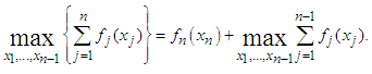 | (4) |
 the equation is independent of
  , and the maximization is taken over non-negative integers
  satisfying
 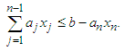 Now,
Now,  for non-negative integers satisfying 2.4 depends on
  or more specifically on
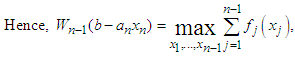 | (5) |
Computing 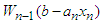 for every allowable value of
 | (6) |
And  can take on the values
 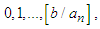 where
where  is the largest integer less than or equal to,
  [15].
[15].  is an investment assigned to the item n, and it is to be chosen based on the minimum value of the correlation of the item n.
 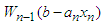 is a function to be maximized over the variables
  . Ideally what we seek to do, in effect, is to take advantage of the recursive relationship then solve from
  of the first stage and finally solve
  which is the maximum return on the issue, while portfolio allocation scheme is also optimal.
3. Theory
Modern Portfolio Theory pointed out that stocks with close correlation should be disregarded. MPT is first adopted in choosing the right stocks (i.e. those stocks with minimum correlation values) to invest. Secondly, our method is applied to the financial problem to obtain the estimated amount of the return achieved. We tested our method by solving the financial problem in the work of [3] and arrived at the same optimal return. We then further modified Bellman’s model and used the tabular-method to resolve it in order to achieve our set objectives. Modern Portfolio Theory (MPT) emphasizes on utilizing the best returns with the least amount of risk on portfolios on different asset risk, but this depends on how one splits up his investment pie. MPT states that if two or more securities have the same weight, one or more of the combined values of these is as good as any other. Analytically, suppose there are  securities; Let
  be the anticipated return at time t per ringgit invested in security
  ; Let
; Let  be the rate at which the return on the
  security selected at time t be discounted back to the present; Let
  be the relative amount invested in security
  . Then the discounted anticipated return of the portfolio is
 Is then the discounted return asset of the
  security.
  Where
Where  is independent of
  Since
Since  for all i and
  is a weighted average of
  with the
  as non-negative weights and to maximize
  , we let
  for
for  with maximum
  . If several
  are maximum, then all allocations with
  [2]. The model on MPT states that: 1) The portfolio of the return is the proportion of the combined weights of the aggregated assets' values.2) The Portfolio volatility is a function of the correlations, ρij of the component assets, for asset pairs (i, j).• Expected return:
 is the return obtained on the portfolio,
  is the return on asset i and,
  is the weighting of component asset
  (that is, the proportion of asset "i" in the portfolio).• Portfolio return variance:
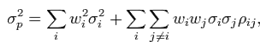 Where
Where  is the correlation coefficient between the returns on assets i and j. Alternatively, the expression can be written as:
 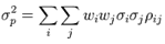 Where
Where  for i = j• Portfolio return volatility (standard deviation):
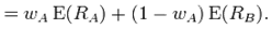
  For a two-asset portfolio: • Portfolio-return;
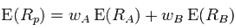
 • Portfolio variance;
  And so continues on the same pattern of combinations for three or more asset.
4. Application to Financial Problem and Result
4.1. Return and Investment Problem
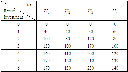
Suppose a company decides to invest RM60, 000 to buy four stocks. The company hopes to confirm the optimal portfolio through a rational allocation of the fund to maximize investment return. After the market investigation and experts forecast, the relationship between return (unit: RM10, 000 per unit) and investment (unit: RM10, 000 per unit) of each stock is as follows:Table 1. Table of Return and Investment Problem
 |
| |
|
4.2. Explanation of the Solution and Results
The recursive solution is calculated from the previous values. The optimum, for instance in table 3, is chosen based on the highest values in the rows that lies between 0 to 6. E.g. between 60, 50 in row 1, 60 is chosen as maximum value. In row 0, no value and so 0 is used. Then out of the maximum values 0, 60, 120, 180, 230, 260 & 280. The highest is 280units which is RM2,800,000. The procedure is applied in all the stages. We have case one which we used to test the model and case two is when we applied  .
.
4.2.1. Case One
In this case, we solve the DP problem of the Bellman’s model without introducing the state control variable  in the model. The model has been modified to suit the dynamic terminologies of the financial problem as follows;
  Therefore, we can get the reverse dynamic programming equation as follow:
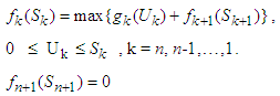 | (7) |
Solving Dynamic Programming Problem of the Model in Tabular Technique (Form);In this case, we regard the process of allocating funds to one or several stocks as a stage. Now we use the "reverse algorithm” of dynamic programming method to solve the whole issue stage by stage. Each figure used in the calculation (table) is in ten thousand per one and their unit in naira has been specified in the problem. We regard the process of allocating funds to one or several stocks as a stage. The First StageGiven  namely investing
 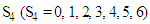 in one stock (the fourth stock), in this case,
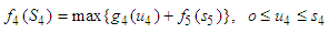
 does not exist at k = 4 since
  is outside the maximum stage
  Obviously, if
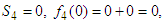
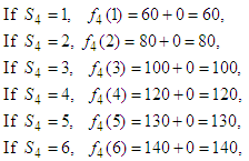
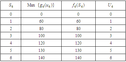
Table 2. Calculation of Optimal Return and Optimal item
 |
| |
|
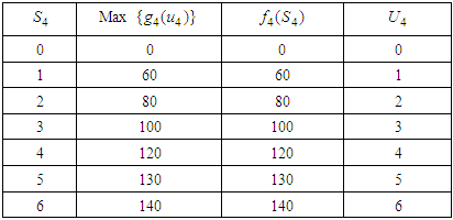
Optimal return at this stage is RM1, 400,000 and the optimal item here is 6.The Second Stage Given  namely investing
 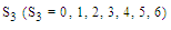 among the two stocks (third and fourth stocks), which makes maximum returns on the investment allocated to the two stocks. In this case,
Table 3. Calculation of Optimal Return and Optimal item
 |
| |
|
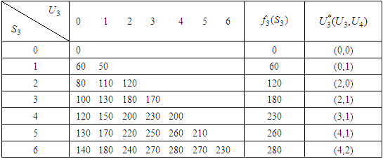
Optimal item, in this case, is ( namely investment allocated to two stocks is 60, 000; including the investment in the fourth stocks is 20, 000, in the third stock is 40, 000. Optimal return at this stage is RM2, 800,000. The Third StageGiven
  namely investing
  among the three stocks (second, third and fourth stocks) which makes a maximum return on the investment allocated to the three stocks. In this case,
  We applied a similar calculation procedure, and then results can be expressed as follows:
 Table 4. Calculation of Optimal Return and Optimal item
 |
| |
|
Optimal item, in this case  is namely investment allocated to the three stocks 60, 000; including investment in the second stock is 20, 000, in the third stock is 30, 000, and in the fourth stock is 10, 000. Optimal return at this time is RM3, 100,000. The Fourth Stage Given
  namely investing
  among the four stocks (first, second, third and fourth stocks) which makes the maximum return on the investment allocated to the four shares.
 Table 5. Calculation of Optimal Return and Optimal Item
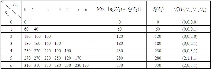 |
| |
|
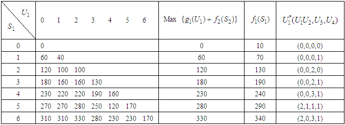
In this case, We apply the same calculation method, and then the results expressed as follows;Optimal item, in this case
  namely investment allocated to the four stocks, is 60, 000; including investment in the first stock is 20, 000, in second stock is 0, in the third stock is 30, 000, in the fourth stock is 10, 000. Optimal return at this time is RM3, 300,000.
4.2.2. Case Two
We solve the DP problem of Bellman's model with the introduction of the state control variable  in the model.
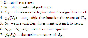 8.
8.  – state control variables. Where
  is a fixed value (arbitrary value) and
  varies at a different stage, e.g. at the first stage,
  = 4 is maximum and k = 5, is an outlier at stage one.Therefore, we can get the reverse dynamic programming equation as follow:
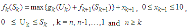 | (8) |
If 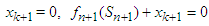 . We will get back to the original equation. The subscripts k represents stages, and the maximum stage in this problem is
  which implies that every calculation outside this range is automatically 0 (give,
  ). The value of k is a chosen value for a particular problem; it is determined by the value of
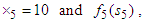
  Solving the Modified Dynamic Programming Model in Table Form; In this case, we regard the process of allocating funds to one or several stocks as a stage. Now we use the "reverse algorithm" of dynamic programming method to solve the whole issue stage by stage. We assume
  = ten and
  = four at every state of all the stages. Recall that
  determines the value of k at every stage.The First StageGiven
  namely investing
 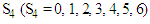 in one stock (the fourth stock), in this case,
 does not exist at k =4 since
  and are outside the maximum stage.
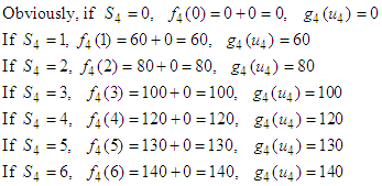
Table 6. Calculation of Optimal Return and Optimal item
 |
| |
|
Optimal return at this stage is RM1, 400,000 and the optimal item here is: 6.The Second Stage Given  namely investing
  among the two stocks (third and fourth stocks), which makes maximum returns on the investment allocated to the two stocks. In this case,
  Optimal item, in this case, is (
 namely investment allocated to two stocks is 60, 000; including investment in the fourth stocks is 20, 000, in the third stock is 40, 000. Optimal return at this stage is RM2, 900,000.
 Table 7. Calculation of Optimal Return and Optimal item
 |
| |
|
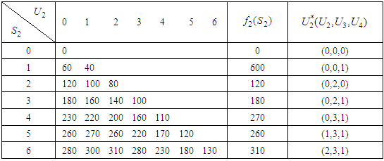
The Third StageGiven  namely investing
  among the three stocks (second, third and fourth stocks) which makes the maximum return on the investment allocated to the three stocks. In this case,
 We applied the same calculation method, and then the results can be expressed as follows;
Table 8. Calculation of Optimal Return and Optimal item
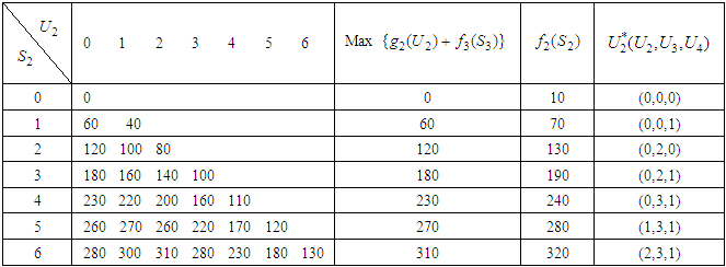 |
| |
|
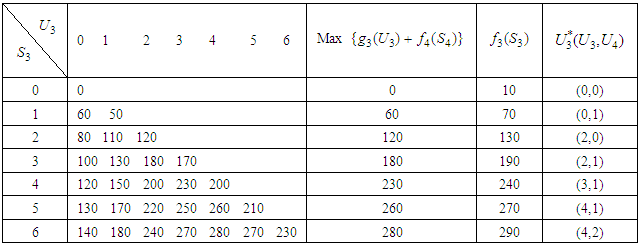
Optimal item, in this case 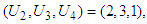 is namely investment allocated to the three stocks 60, 000; including investment in the second stock is 20, 000, in the third stock is 30, 000, and in the fourth stock is 10, 000. Optimal return at this time is RM3, 200,000. The Fourth StageGiven
  namely investing
  among the four stocks (first, second, third and fourth stocks) which makes the maximum return on the investment allocated to the four stocks.
Table 9. Calculation of Optimal Return and Optimal Item
 |
| |
|
In this case,  We applied the same calculation method, and then the results can be expressed as follows;Optimal item, in this case
  is namely investment allocated to the four stocks is 60, 000; including investment in the first stock is 20, 000, in second stock is 0, in the third stock is 30, 000, in the fourth stock is 10, 000. Optimal return at this time is RM3, 400,000 compare with RM3, 300,000 which is the optimal return obtained using the general reverse algorithm of dynamic programming. We called this value, RM3, 400,000, an optimal global result in this research because it gives the highest/best optimal return.
4.3. Network Representation
A network representation of (7) and (8) for both cases is constructed for a clear explanation. Figure 1 shows an example with  = 4 item number of the portfolio. Finding the shortest path from node
  to (1,2,3,4) at stage 4 also gives the optimal sequence in which the stock portfolio should be implemented. Each level (stage) has its maximum item, which produces an optimal return at the stage. The performance in stage 1 is the same as the maximum return of the investment (140) because
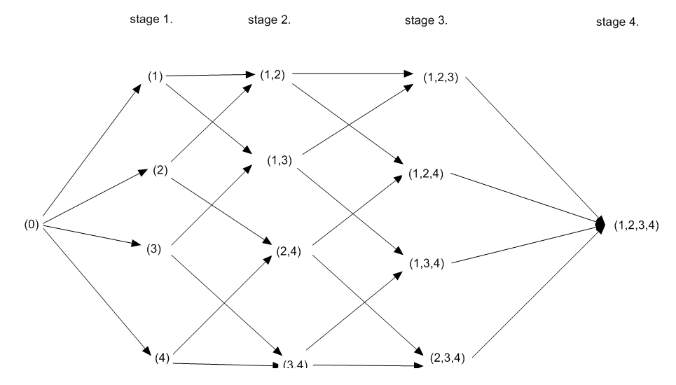 | Figure 1. A network representation for worked example |
Using the Erlenkotter approach, we produced the network diagram shown in Fig. 1. and Fig. 2. The shortest path across this network gives the optimal sequence in which projects should be implemented. In this case, the optimal sequence is to implement stage 1, then stage 2, stage 3, and then stage 4.“The computational advantages of the dynamic programming algorithm are dramatic when compared with the alternative of complete enumeration of all possible sequences. For n items, there are n! possible sequences, each of which might require n discount calculations; however, the dynamic programming method requires only  discount calculations for a complete solution” [16].
5. Conclusions
Given the set of objectives in the study, MPT helped in selection strategies and portfolio diversification techniques. Before investing, the variances and correlation of each stock are calculated, and selection depends on the values. It is safer and wiser to disregard stocks with a close correlation in the selection strategy, according to MPT. Before now investing in a stock without wise choice has ruined lots of investors and companies. Investors are therefore advised to first consult financial experts to guide them in investment strategy by carrying out pilot analysis of what the should expect in their investment. In this study, the company problem was first converted to a dynamic programming problem using suitable terminologies. This work successfully applied a table-like method in the company's financial problem, and the optimal result obtained gives the same result with that of the traditional method. Still, the table-like technique is more uncomplicated in computation when compared. Modification of the model (i.e. introduction of a state control variable) subsequently resulted in a global maximum return (RM3, 400,000). When the modified model was applied to solve the same stock portfolio problem (company's financial problem), the observation was that the optimal performance was improved at each stage except at the first stage, where the rule does not apply: it is outside the chosen range. The final result obtained in the modified model (case two) i.e at the introduction of the control variable, yields the highest optimal result compared to that in the case one (used as test case). Further research is currently ongoing on tracing the paths that leads to global maximum via network representation. The researchers recommend future research on writing the codes that can solve the problem so as to save time more time.
ACKNOWLEDGEMENTS
Thanks to the school of Mathematical Sciences, Universiti Sains Malaysia for financial support for this Conference. Thanks to Department of Statistics, University of Nigeria for training of experienced Staff.
References
| [1] | Hamdy, A.T., Operations research an introduction. 7th ed. 2002, New Jersey: Prentice Hall. |
| [2] | Markowitz, H., Portfolio selection. The journal of finance, 1952. 7(1): p. 77-91. |
| [3] | Yan, F. and F. Bai, Application of dynamic programming model in stock portfolio-under the background of the subprime mortgage crisis. International Journal of Business and management, 2009. 9(3): p. 178-182. |
| [4] | Akinwale, S. and R. Abiola, A conceptual model of asset portfolio decision making: a case study in a developing economy. African Journal of Business Management, 2007. 1(7). |
| [5] | Haugh, M.B. and L. Kogan, Duality theory and approximate dynamic programming for pricing American options and portfolio optimization. Handbooks in operations research and management science, 2007. 15: p. 925-948. |
| [6] | Bellman, R.E. and S.E. Dreyfus, Applied dynamic programming. Vol. 2050. 2015: Princeton University Press. |
| [7] | Polson, N.G. and M. Sorensen, A simulation‐based approach to stochastic dynamic programming. Applied Stochastic Models in Business and Industry, 2011. 27(2): p. 151-163. |
| [8] | Fang, J., et al., Sourcing strategies in supply risk management: An approximate dynamic programming approach. Computers & Operations Research, 2013. 40(5): p. 1371-1382. |
| [9] | Richard, C., Market Value Maximization and Markov Dynamic Programming. Journal of Management Sciences, 1983. Vol. 29: p. 15-32. |
| [10] | Brandt, W., Goyal A., Santa-Clara, P. and Stroud, R, A Simulation Approach to Dynamic Portfolio Choice with an Application to Learning About Return Predictability. Society of finance Study., 2003. Vol 18: p. pp. 835-838. |
| [11] | Vulcano, G., G. Van Ryzin, and C. Maglaras, Optimal dynamic auctions for revenue management. Management Science, 2002. 48(11): p. 1388-1407. |
| [12] | Yao, D.D., S. Zhang, and X.Y. Zhou, Tracking a financial benchmark using a few assets. Operations Research, 2006. 54(2): p. 232-246. |
| [13] | Yusuf, I. and N. Christopher, I,(2012), The modern portfolio theory as an investment decision tool. Journal of Accounting and Taxation, 2012. 4(2): p. 19-28. |
| [14] | Sankar, K., Mathematical Programming and Game Theory for Decision Making, 2008. Vol. 1: p. pp. 2-13. |
| [15] | Hadley, G., Nonlinear and Dynamic Programming. 1st edition ed, ed. F. edition. 1964, New York city. USA: Addison-Wesley publishing Inc. |
| [16] | Vanberkel, P.T., et al., Optimizing the strategic patient mix combining queueing theory and dynamic programming. Computers & operations research, 2014. 43: p. 271-279. |

 Abstract
 Reference
 Full-Text PDF
 Full-text HTML